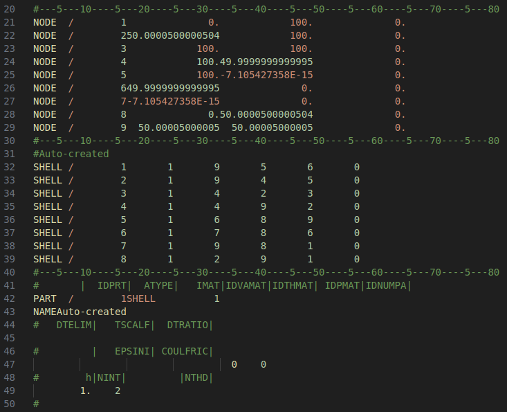
Reading all the contents of a file is straightforward, but “parsing” a file can require some effort, i.e. when you want to extract specific parts based on the structure of the contents. The following is an example of how this can be done for a certain file format that uses fixed width formatting.
(a) File structure to be parsed
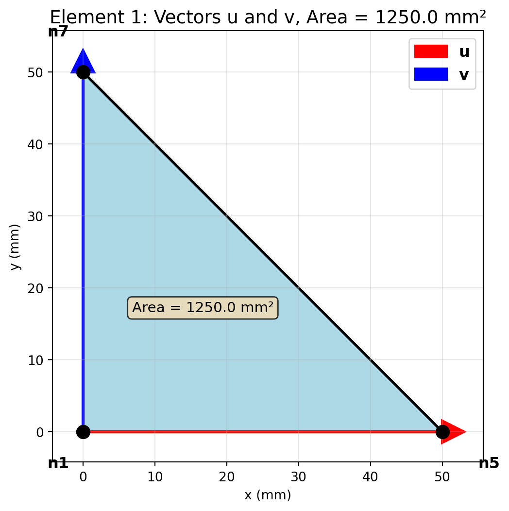
(b) Visualization of finite element mesh
Figure 8.7.1: Example file contents and the geometry it represents.
The example file describes a two-dimensional finite element mesh consisting of eight connected triangles. We are interested in computing the total area of the geometry. To do this, we first need to parse all lines starting with NODE and SHELL from the file, then compute the area of each individual triangle. All other lines in the file are not of interest, and should be ignored.
The code below initializes two empty lists: node_coords and connectivity, then loops over each line of the file. Data is only appended to each list if a line begins with NODE or SHELL. We use .split() to separate each line into parts by whitespace, making it easy to extract the values by index. Casting is used to specify the data type of each collected variable (int for IDs, float for coordinates).
After parsing, we create a Mesh object from MechanicsKit, which provides a clean interface with 1-based node numbering (matching the file format). This eliminates the need for manual index translation.
For SHELL lines, we extract the node IDs that define each triangular element. Note that these are 1-based indices (node numbering starts at 1, not 0), which the file format uses. The Mesh class handles this 1-based indexing naturally.
Computing the area
Since we know the x-, y- and z-coordinates of each node in every element, we can utilize linear algebra to compute the area from the vector product of the element sides. Recall that the vector product \(\mathbf{u} \times \mathbf{v}\) is a new vector \(\mathbf{w}\) (perpendicular to both \(\mathbf{u}\) and \(\mathbf{v}\)) whose magnitude \(||\mathbf{w}|| = \sqrt{w_x^2 + w_y^2 + w_z^2}\) represents the area of the parallellogram defined by \(\mathbf{u}\) and \(\mathbf{v}\) as sides. The area of a triangular element is therefore \(A_i = \frac{1}{2}||\mathbf{w}||\).
The Mesh class makes accessing node coordinates simple with mesh.get_node(), which uses natural 1-based numbering. We can iterate over elements using mesh.iter_elements(), which yields tuples of (element_number, node_IDs, node_coordinates) for each element.
Code
# Compute total areaarea =0for iel, nodes, coords in mesh.iter_elements():# iter_elements() yields: element_number, node_IDs, node_coordinates# Extract the three node coordinates for this triangular element n1 = coords[0] # first node coordinates n2 = coords[1] # second node coordinates n3 = coords[2] # third node coordinates# Compute edge vectors and area u = n2 - n1 # triangle edge vector 1 v = n3 - n1 # triangle edge vector 2 w = np.cross(u, v) # perpendicular to triangle area_e =0.5* np.linalg.norm(w) # area of current element area += area_e # add to total areaprint(f"Total computed area: {area:.2f} mm²")print(f"Expected area: {100*100:.2f} mm² (100mm × 100mm square)")print(f"Verification: Error = {abs(area -10000):.6f} mm²")
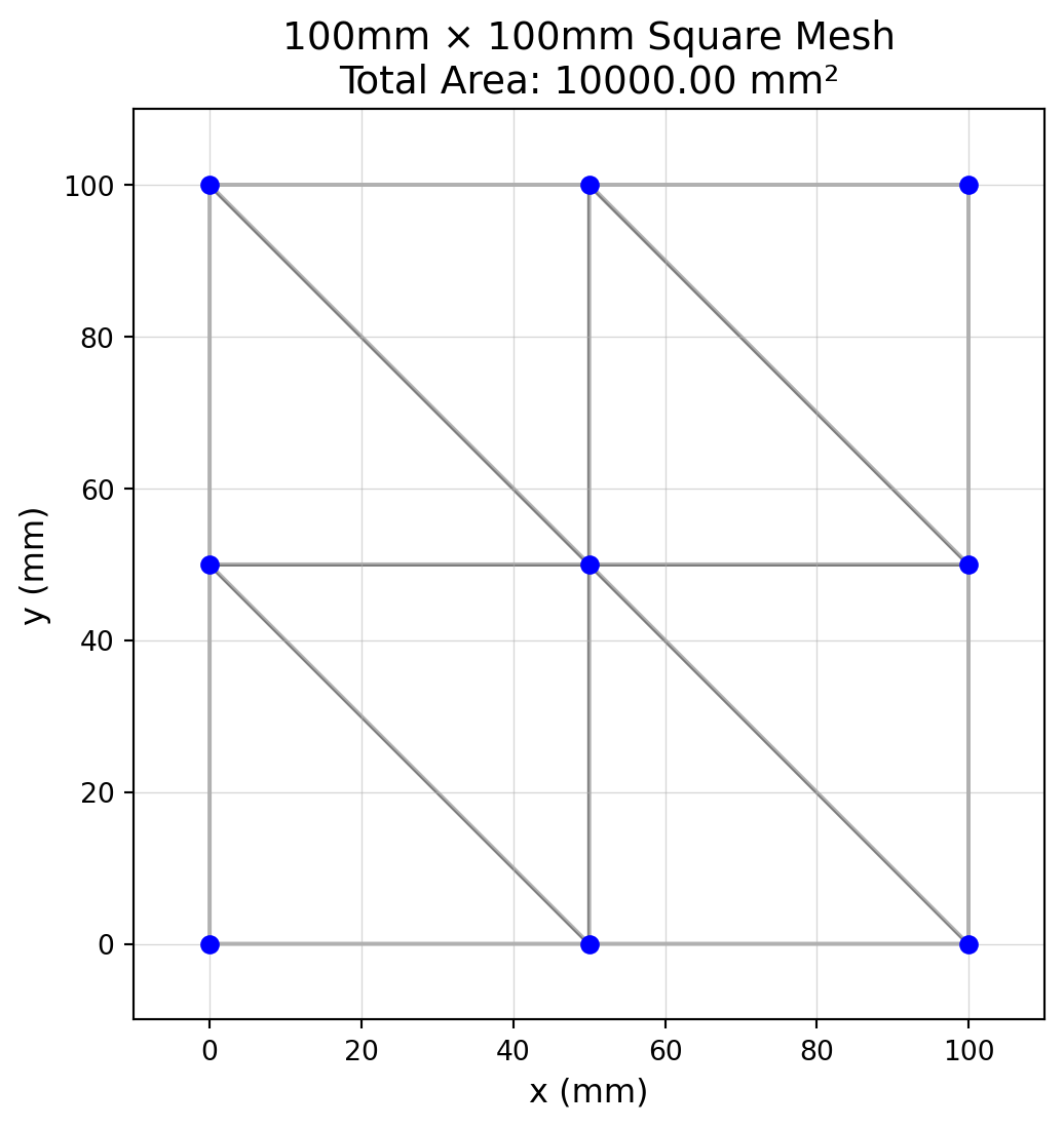
Now let’s visualize the entire mesh to verify the geometry and area:
Code
# Prepare data for patch function using MeshP = mesh.nodes[:, :2] # Extract x, y coordinates from Mesh# Visualize meshfig, ax = plt.subplots(figsize=(6, 6))# Plot mesh with semi-transparent white faces and black edgesmk.patch('Faces', mesh.elements, 'Vertices', P,'FaceColor', 'white','EdgeColor', 'black','EdgeAlpha', 0.3,'LineWidth', 1.5, ax=ax)# Plot nodesax.plot(P[:, 0], P[:, 1], 'o', color='blue', markersize=6)# Add grid for area verificationax.grid(True, alpha=0.5, linewidth=0.5)ax.set_aspect('equal')ax.set_xlim(-10, 110)ax.set_ylim(-10, 110)ax.set_xlabel('x (mm)', fontsize=12)ax.set_ylabel('y (mm)', fontsize=12)ax.set_title(f'100mm × 100mm Square Mesh\nTotal Area: {area:.2f} mm²', fontsize=14)plt.show()
The visualization clearly shows the 100mm × 100mm square mesh. The grid helps verify the dimensions, and the computed area of 10000 mm² matches the expected area perfectly.
The *ELEMENT_SHELL section supports both triangular and quadrilateral elements. Triangular elements are represented by repeating the last node. For example:
Element 1: 210 180 181 181 - This is a triangle with nodes 210, 180, and 181 (node 181 repeated)
Element 2: 180 80 81 81 - This is a triangle with nodes 180, 80, and 81 (node 81 repeated)
This convention allows the file format to use a fixed 4-node format for both element types.
Thus we need a different way of parsing this.
Parsing the .k file
The .k file format uses fixed-width columns for node data and space-separated values for element data. Unlike the previous format, node coordinates can run together without spaces (especially when negative), requiring careful column-based parsing.
Code
# Parse circle mesh from .k filenode_dict = {} # Map node ID to coordinatesconnectivity_circle = []# Track which section we're inin_node_section =Falsein_element_section =Falsewithopen('../assets/unit_circle_cirk_pattern.k', 'r') asfile:for line infile:# Check for section headersif line.startswith('*NODE'): in_node_section =True in_element_section =Falsecontinueelif line.startswith('*ELEMENT_SHELL'): in_node_section =False in_element_section =Truecontinueelif line.startswith('*'):# New section started, stop parsing in_node_section =False in_element_section =Falsecontinue# Parse node data (fixed-width format)if in_node_section and line.strip():# Fixed-width columns: 8 chars for ID, 16 chars each for X, Y, Z NID =int(line[0:8]) NX =float(line[8:24]) NY =float(line[24:40]) NZ =float(line[40:56]) node_dict[NID] = [NX, NY, NZ]# Parse element data (space-separated)elif in_element_section and line.strip(): parts = line.split() EID =int(parts[0])# Column 1 is material/property ID, columns 2-4 are the three unique node IDs# (Column 5 repeats the last node for triangular elements) N1 =int(parts[2]) N2 =int(parts[3]) N3 =int(parts[4]) connectivity_circle.append([N1, N2, N3])# Build sequential node coordinate list and update connectivity to match# Map original node IDs to sequential indices (1-based for Mesh class)node_id_to_index = {nid: idx+1for idx, nid inenumerate(sorted(node_dict.keys()))}node_coords_circle = [node_dict[nid] for nid insorted(node_dict.keys())]# Remap connectivity from original node IDs to sequential indicesconnectivity_remapped = [[node_id_to_index[n1], node_id_to_index[n2], node_id_to_index[n3]]for n1, n2, n3 in connectivity_circle]# Create Mesh object with 1-based indexingmesh_circle = mk.Mesh(node_coords_circle, connectivity_remapped)print(f"Circle mesh: {mesh_circle.n_nodes} nodes, {mesh_circle.n_elements} elements")print(f"Node ID range: {min(node_dict.keys())} to {max(node_dict.keys())}")
Circle mesh: 209 nodes, 387 elements
Node ID range: 1 to 360
Parsing explained
The .k file format presents two main challenges that require different parsing strategies than the previous example:
Challenge 1: Fixed-width columns with no separators
Unlike the .pc format where values are separated by spaces, the .k format uses fixed-width columns:
1-.80556840782042-.59143545453769 0. 0 0
Notice how the node ID (1) runs directly into the x-coordinate (-0.805…), which runs into the y-coordinate (-0.591…). Using .split() wouldn’t work here.
This extracts data from specific column positions regardless of spacing.
Challenge 2: Non-sequential node IDs
The file contains node IDs like 1, 2, 4, 5, 6, 7, 8, 9, 10, … 188, …, 360 (with gaps). Elements reference these actual IDs:
1 1 210 180 181 181
This element uses nodes 210, 180, and 181.
If we simply append coordinates to a list, we lose the node ID mapping and can’t resolve these references.
Solution: Dictionary mapping and remapping
The Mesh class requires sequential node numbering (1, 2, 3, …, n_nodes). We need to convert the file’s non-sequential IDs into sequential indices.
The parsing code above uses list comprehensions and dictionary comprehensions for conciseness. Below, we explain the same logic using for loops, which are more explicit and easier to follow when learning Python:
# Step 1: Store coordinates by node ID during parsingnode_dict[NID] = [NX, NY, NZ]# e.g., node_dict[1] = [x1, y1, z1], node_dict[210] = [x210, y210, z210]# Step 2: Create sequential coordinate list and ID-to-index mappingsorted_ids =sorted(node_dict.keys()) # [1, 2, 4, 5, ..., 210, ..., 360]# Build mapping: original node ID → new sequential indexnode_id_to_index = {}for idx, nid inenumerate(sorted_ids): node_id_to_index[nid] = idx +1# Now: node 1 → index 1, node 2 → index 2, node 4 → index 3, node 210 → index 50, etc.# Build sequential coordinate list in same ordernode_coords_circle = []for nid in sorted_ids: node_coords_circle.append(node_dict[nid])# Step 3: Remap connectivity from file IDs to sequential indicesconnectivity_remapped = []for n1, n2, n3 in connectivity_circle: new_n1 = node_id_to_index[n1] new_n2 = node_id_to_index[n2] new_n3 = node_id_to_index[n3] connectivity_remapped.append([new_n1, new_n2, new_n3])# Example: element with nodes [210, 180, 181] → [50, 45, 46]
Note
The actual parsing code uses these equivalent one-line expressions:
# Dictionary comprehension (equivalent to the for loop building node_id_to_index)node_id_to_index = {nid: idx+1for idx, nid inenumerate(sorted(node_dict.keys()))}# List comprehension (equivalent to the for loop building node_coords_circle)node_coords_circle = [node_dict[nid] for nid insorted(node_dict.keys())]# Nested list comprehension (equivalent to the for loop building connectivity_remapped)connectivity_remapped = [[node_id_to_index[n1], node_id_to_index[n2], node_id_to_index[n3]]for n1, n2, n3 in connectivity_circle]
Both approaches produce identical results; comprehensions are more compact while for loops make each step explicit.
This remapping is required because the Mesh class uses sequential indexing internally (accessing node N means getting nodes[N-1] from the array).
Section tracking
The file uses section headers (*NODE, *ELEMENT_SHELL) to organize data. We use boolean flags to track which section we’re currently parsing:
This ensures we apply the correct parsing logic to each line based on its section.
Visualizing the mesh
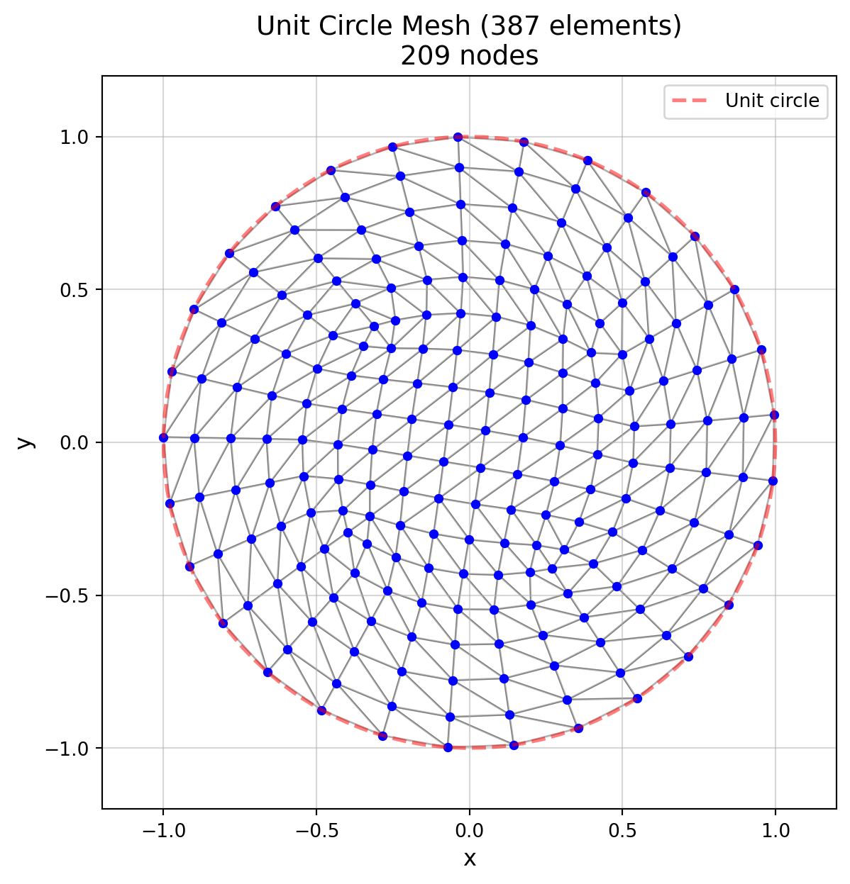
Let’s visualize the circle mesh to verify the geometry:
Code
# Prepare data for visualization using MeshP_circle = mesh_circle.nodes[:, :2] # Extract x, y coordinates from Mesh# Visualizefig, ax = plt.subplots(figsize=(7, 7))# Plot mesh using mesh.elements (1-based connectivity) directlymk.patch('Faces', mesh_circle.elements, 'Vertices', P_circle,'FaceColor', 'white','EdgeColor', 'black','EdgeAlpha', 0.3,'LineWidth', 1.0, ax=ax)# Plot nodesax.plot(P_circle[:, 0], P_circle[:, 1], 'o', color='blue', markersize=4)# Add grid for verificationax.grid(True, alpha=0.5)ax.set_aspect('equal')ax.set_xlim(-1.2, 1.2)ax.set_ylim(-1.2, 1.2)# Draw unit circle outline for referencetheta = np.linspace(0, 2*np.pi, 100)ax.plot(np.cos(theta), np.sin(theta), 'r--', linewidth=2, alpha=0.5, label='Unit circle')ax.set_xlabel('x', fontsize=12)ax.set_ylabel('y', fontsize=12)ax.set_title(f'Unit Circle Mesh ({mesh_circle.n_elements} elements)\n'+f'{mesh_circle.n_nodes} nodes', fontsize=14)ax.legend()plt.show()
The circle mesh visualization shows a well-structured triangular mesh that approximates the unit circle.
Computing the area
Code
# Compute area using Mesh classarea_circle =0for iel, nodes, coords in mesh_circle.iter_elements():# iter_elements() yields: element_number, node_IDs, node_coordinates# Extract the three node coordinates for this triangular element n1 = coords[0] n2 = coords[1] n3 = coords[2]# Compute edge vectors and area u = n2 - n1 v = n3 - n1 w = np.cross(u, v) area_e =0.5* np.linalg.norm(w) area_circle += area_eprint(f"\nTotal computed area: {area_circle:.6f}")print(f"Expected area (π × r²): {np.pi:.6f}")print(f"Verification: Error = {abs(area_circle - np.pi):.6f}")print(f"Relative error: {100*abs(area_circle - np.pi) / np.pi:.4f}%")
Total computed area: 3.116674
Expected area (π × r²): 3.141593
Verification: Error = 0.024919
Relative error: 0.7932%
The computed area is slightly smaller than π. This is expected because the triangular mesh approximates the circle’s curved boundary with straight edges. When mesh nodes lie on the circle’s circumference, the straight edges connecting them form chords that cut across the circle, excluding the small curved segments between each chord and the arc. The finer the mesh (more elements along the boundary), the closer the computed area would be to the true value of π. This demonstrates how linear elements directly affect geometric accuracy in finite element analysis. Another approach would be to utilize higher-order elements, essentially curved elements, to better capture the geometry. In that case, the geometric error could be zero even with far fewer elements!