7.8  2D Interpolation - Bi-linear Shape Functions

Visualizing the Element and Nodal Values

We start by defining the geometry of a single quadrilateral element with four nodes. The coordinates of the nodes are stored in a matrix P, and a scalar value (e.g., temperature) at each node is stored in a vector U.

# Nodal coordinates (4 nodes, 2 dimensions)
P = np.array([[0.0, 0.0],   # Node 1
              [1.0, 0.0],   # Node 2
              [0.9, 1.0],   # Node 3
              [-0.1, 1.2]]) # Node 4

# Nodal values (e.g., temperature)
U = np.array([20, 30, 40, 25])

# Element connectivity (a single quad element)
# Using 1-based indexing as is common in FEM
faces = np.array([[1, 2, 3, 4]])

We can visualize this element and the scalar field using the patch function from MechanicsKit. By setting FaceColor to 'interp', the function will interpolate the nodal values (CData) across the face of the element.

fig, ax = plt.subplots(figsize=(7, 6))

mk.patch(Faces=faces, Vertices=P, CData=U, FaceColor='interp', cmap='jet')

mk.colorbar(label='Nodal Value (e.g., Temperature)')

ax.plot(P[:, 0], P[:, 1], 'ok', markerfacecolor='k')

ax.set(aspect='equal',
       title='Quadrilateral Element with Interpolated Nodal Values',
       xlabel='X-coordinate',
       ylabel='Y-coordinate',
       xlim=[-0.2, 1.1],
       ylim=[-0.1, 1.3])
plt.show()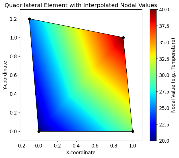

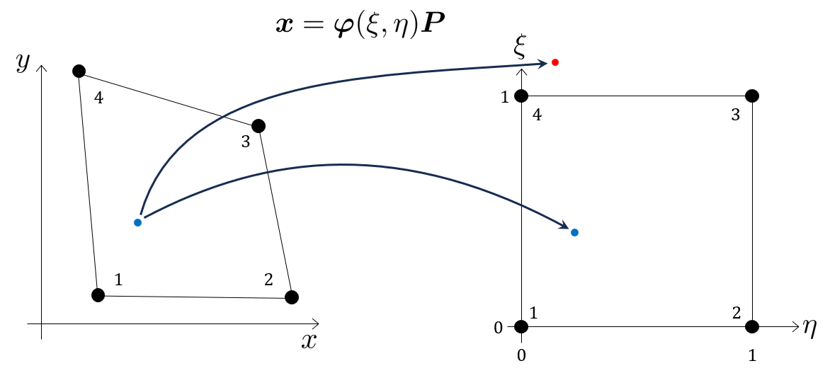
Basis Functions in Parametric Coordinates

Now, we want to know what the value \(u_h\) is inside the element at the point \((x,y)\).

The interpolation is performed using basis functions (or shape functions) defined in a local, parametric coordinate system (ξ, η), which ranges from 0 to 1. For the quadrilateral element, the bi-linear basis functions defined in the parametric coordinates \(\xi, \eta \in [0,1]\):

\[ \varphi(\xi, \eta)=\left[\begin{array}{c} (1-\xi)(1-\eta) \\ \xi(1-\eta) \\ \xi \eta \\ \eta(1-\xi) \end{array}\right]^{\mathsf{T}} \]

xi, eta = sp.symbols('xi eta')

# Define the basis functions as a list of symbolic expressions
phi_sym_list = [
    (1 - xi) * (1 - eta),  # phi1
    xi * (1 - eta),        # phi2
    xi * eta,              # phi3
    (1 - xi) * eta         # phi4
]

# Convert to a sympy Matrix for easier manipulation
phi_sym = sp.Matrix(phi_sym_list).T # Transpose to a row vector

Interpolating the Scalar Field

The interpolated value Uh at any point \((ξ, η)\) inside the element is a weighted average of the nodal values U, where the weights are the basis functions:

\[ U_h(\xi, \eta) = \sum_{i=1}^{4} \varphi_i(\xi, \eta) U_i = \boldsymbol{\varphi}(\xi, \eta) \mathbf{U} \]

# Perform the symbolic interpolation
U_sym = sp.Matrix(U)
Uh_sym = phi_sym * U_sym
Uh_sym = sp.simplify(Uh_sym[0])

Ok, so now we can evaluate the values somwhere inside element, but only in parametric coordinates. For instance in the midpoint we have \(u_h(\xi=0.5, \eta=0.5)\):

Uh_sym.subs({xi:0.5, eta:0.5})

Mapping from Physical to Parametric Coordinates - Affine elements

The issue is when we actually want the values \(u_h\) as functions of the coordinates \(x, y\), i.e., \(u(x, y)\), we need to solve a system of equations which, depending on the geometry of the element (the coordinates \(\mathbf{P}\) ), will be either linear or non-linear. For instance when \(\mathbf{P}\) is affine:

P = np.array([[0,0],
              [2,0],
              [2,1],
              [0,1]])

fig, ax = plt.subplots(figsize=(7, 6))
mk.patch(Faces=np.array([[1,2,3,4]]), Vertices=P, FaceColor='w')
ax.plot(P[:, 0], P[:, 1], 'ok', markerfacecolor='k')
ax.set(aspect='equal')
plt.show()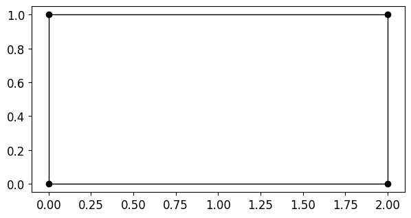

We want to solve the linear system:

\[ \boldsymbol{\varphi}(\xi, \eta) \mathbf{P} = \left[\begin{array}{c} x \\ y \end{array}\right] \]

for \(\xi(x, y)\) and \(\eta(x, y)\).

x,y = sp.symbols('x y')

eqs = sp.Eq((phi_sym*P).T, sp.Matrix([[x, y]]).T ).simplify()

We see that this system is trivial to solve for affine elements:

sol = sp.solve(eqs, (xi, eta))

We can then substitute \(\xi(x, y)\) and \(\eta(x, y)\) into \(\boldsymbol \varphi(\xi, \eta)\) to get the basis functions as functions of \(x\) and \(y\), \(\boldsymbol \varphi (x, y)\):

phi_sym_1 = phi_sym.subs({xi: sol[xi], eta: sol[eta]})
phi_sym_1 = sp.simplify(phi_sym_1).T

Which we can use as an interpolant for \(u_h(x, y)\):

\[ \boxed{ u_h(x, y) = \boldsymbol{\varphi}(x, y) \mathbf{U} } \]

Mapping from Physical to Parametric Coordinates - Non-Affine elements

If, however, the element is non-affine, e.g.,

P = np.array([[0,0],
              [1,0],
              [0.9,1],
              [-0.1,1.2]])

fig, ax = plt.subplots(figsize=(7, 6))
mk.patch(Faces=np.array([[1,2,3,4]]), Vertices=P, FaceColor='w')
ax.plot(P[:, 0], P[:, 1], 'ok', markerfacecolor='k')
ax.set(aspect='equal')
plt.show()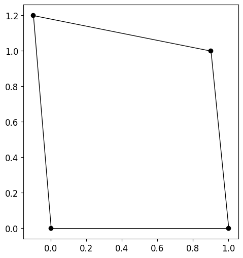

using \(\varphi(\xi, \eta) \mathbf{P}=[x, y]\) and solving again for \(\xi(x, y)\) and \(\eta(x, y)\) we get the non-linear system of equations

x, y = sp.symbols('x y')
P_sym = sp.Matrix(P)

# System of equations: phi * P = [x, y]
eqs = sp.Eq( (phi_sym * P_sym).T, sp.Matrix([[x, y]]).T ).simplify()
eqs

notice how we can not formulate a system of the form \(\mathbf A \xi + \mathbf B \eta + \mathbf C = 0\). We can however solve this system using sympy:

sol = sp.solve(eqs, (xi, eta), dict=True)

here, in the two solutions \(\xi_1(x, y)\) and \(\xi_2(x, y)\), only one is within the valid parametric space \(\xi, \eta \in[0,1]\), which is \(\xi_1\) and \(\eta_1\) (after testing).

xi1 = sol[0][xi]
eta1 = sol[0][eta]
phi_sym_xy = phi_sym.subs({xi: xi1, eta: eta1})
phi_sym_xy = sp.simplify(phi_sym_xy)

phi_np = sp.lambdify((x, y), phi_sym_xy, 'numpy')
phi_np(P[:,0], P[:,1])[0] | la

Here we just verify that the mapping is correct by evaluating the corner points. We get back an identity matrix as expected. Since the basis functions are one in “their” nodes and zero in all other nodes.

For our problem where we want to generate the function \(u_h(x, y)\), we can now use \(u_h(x, y)=\varphi(x, y) \mathbf{U}\)

U_sym

phi_sym_xy.T

x, y = sp.symbols('x y')
Uh_sym_xy = (phi_sym_xy * U_sym)[0]

Evaluating this function at a known point, e.g., \(x=0\), \(y=0\), we get back the expected nodal value \(U=20\).

Uh_sym_xy.subs({x:0.0, y:0.0})

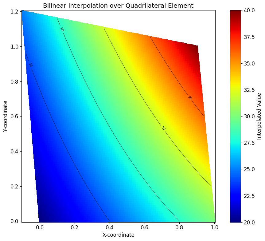
Visualizing the Interpolated Field

Now we can visualize the interpolated scalar field \(U_h\) over the physical domain of the element. We create a grid of points in the parametric (ξ, η) space, map these points to the physical (x, y) space, and evaluate the interpolated function \(U_h\) at each point.

# Create a grid in the parametric space
N = 100
xi_vals = np.linspace(0, 1, N)
eta_vals = np.linspace(0, 1, N)
Xi, Eta = np.meshgrid(xi_vals, eta_vals)

# Lambdify the symbolic basis functions for numerical evaluation
# We need to evaluate phi for each point in the grid
phi_func = sp.lambdify((xi, eta), phi_sym, 'numpy')

# Evaluate - returns shape (1, 4) for each point, but numpy broadcasts
Phi = phi_func(Xi.ravel(), Eta.ravel())  # Shape: (1, 4, N*N)
Phi = np.squeeze(Phi)  # Now shape: (4, N*N)

UH = (Phi.T @ U).reshape(N, N)

PP = Phi.T @ P # Shape: (N*N, 2)
X = PP[:, 0].reshape(N, N)
Y = PP[:, 1].reshape(N, N)

# Plot
fig, ax = plt.subplots(figsize=(10, 8))
surf = ax.pcolormesh(X, Y, UH, cmap='jet', shading='auto')
contours = ax.contour(X, Y, UH, levels=5, colors='k', linewidths=0.5)
ax.clabel(contours, inline=True, fontsize=8)
ax.set_aspect('equal')
ax.set_xlabel('X-coordinate')
ax.set_ylabel('Y-coordinate')
ax.set_title('Bilinear Interpolation over Quadrilateral Element')
plt.colorbar(surf, ax=ax, label='Interpolated Value')
plt.tight_layout()
plt.show()