In many fields of engineering and scientific visualization, it is necessary to represent scalar data defined at the vertices of a polygon with a smooth, interpolated color fill. A common tool for this task is MATLAB, which handles such requirements with its patch function. We begin with a representative example in MATLAB, where a quadrilateral is defined by four vertices P and a scalar value U is assigned to each vertex.
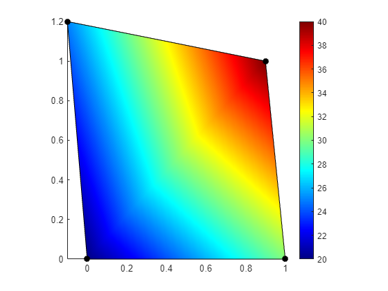
The interpolated shading is achieved through the 'FaceColor', 'interp' argument, which instructs the program to interpolate the CData values across the face of the polygon. This process results in a smooth gradient that accurately represents the data variation, as shown in the figure below.
The target MATLAB plot with smooth color interpolation across a quadrilateral.
Our objective is to replicate this behavior in Python using the Matplotlib library. This exploration, while appearing straightforward, will reveal a fundamental trade-off between computational performance and visual fidelity, highlighting important details about how different rendering methods operate.
Approach 1: Direct Rendering with tripcolor
A direct approach for plotting on an arbitrary polygon in Matplotlib is to first decompose it into a set of triangles, a process known as triangulation. Once we have a triangulated mesh, we can employ a function designed for such meshes. The most direct tool for this purpose is ax.tripcolor. When combined with the shading='gouraud' argument, this function instructs the rendering backend to perform linear interpolation of the color at each vertex across the face of the triangle. This method is performant and memory-efficient because it passes the geometry directly to the renderer, often leveraging hardware acceleration.
A quadrilateral, however, can be triangulated in two ways by choosing either of its two internal diagonals. Let us consider the case where we split the quad along the diagonal connecting vertices v0 and v2.
Code
# quad_tripcolor_diagonal_v0v2.pyimport numpy as npimport matplotlib.pyplot as pltfrom matplotlib.tri import Triangulation# Data for the original quadrilateralP_verts = np.array([ [0, 0], # v0 [1.0, 0], # v1 [0.9, 1.0], # v2 [-0.1, 1.2] # v3])U_vals = np.array([20, 30, 40, 25])x, y = P_verts[:, 0], P_verts[:, 1]# Triangulation using the (v0-v2) diagonaltriangles = [[0, 1, 2], [0, 2, 3]]triang = Triangulation(x, y, triangles=triangles)# --- Plotting ---fig, ax = plt.subplots()tpc = ax.tripcolor(triang, U_vals, cmap='jet', shading='gouraud', vmin=U_vals.min(), vmax=U_vals.max())ax.set_aspect('equal')ax.axis('tight')fig.colorbar(tpc, ax=ax)plt.show()
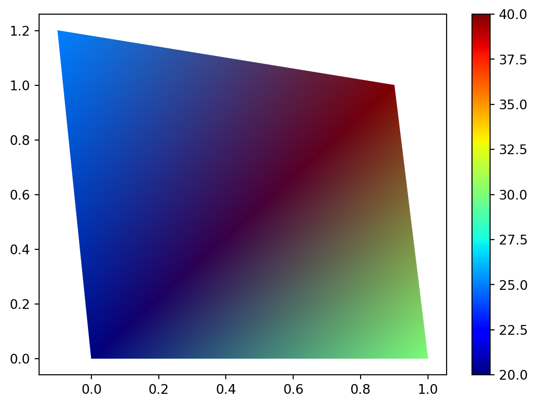
The resulting plot, appears reasonable at first glance. However, it exposes a limitation of this direct approach.
tripcolor performs a mathematically linear interpolation of the data values over each triangle. Linear as in taking the nodal values and interpolating linearly between them. The interpolated values do not correspond to the colormap as we can clearly see. We expect the line between node 1 and 3 (lower left and upper right corners) to be colored according to the colormap and look exactly like the colorbar. Which clearly is not the case!
Approach 2: Smoothed Rendering with tricontourf
To obtain a visually more accurate gradient that more closely matches the MATLAB output, we now consider an alternative method, ax.tricontourf. This function operates not by rendering the geometric primitives directly, but by first creating a fine raster grid and interpolating the vertex data onto it. The crucial step is that it then calculates the regions between a large number of contour levels. Each of these regions is filled with a single solid color sampled from the colormap. By specifying many levels, we simulate a near-continuous gradient. This process effectively honors the (often non-linear) color transitions of the colormap itself, producing the desired visual result.
Code
# quad_tricontourf_diagonal_v0v2.pyimport numpy as npimport matplotlib.pyplot as pltfrom matplotlib.tri import TriangulationP_verts = np.array([ [0, 0], [1.0, 0], [0.9, 1.0], [-0.1, 1.2]])U_vals = np.array([20, 30, 40, 25])x, y = P_verts[:, 0], P_verts[:, 1]triangles = [[0, 1, 2], [0, 2, 3]]triang = Triangulation(x, y, triangles=triangles)fig, ax = plt.subplots()# Using many levels gives a smoother appearance at a performance cost.levels = np.linspace(U_vals.min(), U_vals.max(), 256)cf = ax.tricontourf(triang, U_vals, levels=levels, cmap='jet')ax.set_aspect('equal')ax.axis('tight')fig.colorbar(cf, ax=ax)plt.show()
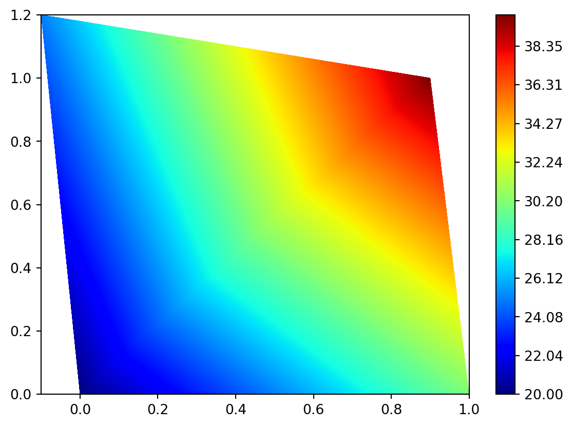
This code produces a result that is visually much closer to the target MATLAB plot. The intermediate gridding and contouring process effectively smooths over the gradient discontinuity at the triangle boundary. This creates the appearance of a continuous, non-linear color transition that follows the fine gradations of the colormap, achieving the desired visual fidelity at the cost of computational performance.
Visualizing the tricontourf Internal Grid
tricontourf creates a fine rectangular grid over the mesh and calculates the color for each grid cell, a process we can simulate.
To visualize this internal mechanism, we can perform the important steps manually:
Create a LinearTriInterpolator from our original mesh and data.
Define a grid (coarse enough for us to see the individual cells) that covers the plot area.
Evaluate the interpolator at each point on our grid.
Plot the resulting grid of values using ax.pcolormesh.
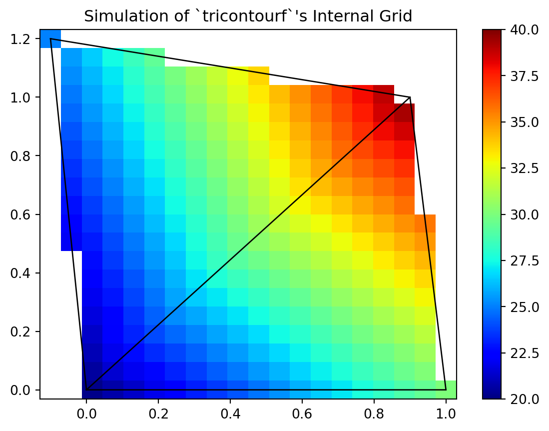
The code below demonstrates this process. The resulting plot reveals the pixelated grid of values that tricontourf uses internally before its final contouring algorithm creates the smooth polygons.
Code
# tricontourf_internal_grid.pyimport numpy as npimport matplotlib.pyplot as pltfrom matplotlib.tri import Triangulation, LinearTriInterpolatorP_verts = np.array([ [0, 0], [1.0, 0], [0.9, 1.0], [-0.1, 1.2]])U_vals = np.array([20, 30, 40, 25])x, y = P_verts[:, 0], P_verts[:, 1]triangles = [[0, 1, 2], [0, 2, 3]]triang = Triangulation(x, y, triangles=triangles)# 1. Create the interpolator objectinterpolator = LinearTriInterpolator(triang, U_vals)# 2. Create a coarse grid to sample the interpolatorn_grid =20xi = np.linspace(x.min(), x.max(), n_grid)yi = np.linspace(y.min(), y.max(), n_grid)Xi, Yi = np.meshgrid(xi, yi)# 3. Evaluate the interpolator on the gridzi = interpolator(Xi, Yi)# --- Plotting ---fig, ax = plt.subplots()# 4. Use pcolormesh to visualize the rasterized data# The blocky pixels represent the data on the internal gridax.pcolormesh(Xi, Yi, zi, cmap='jet', vmin=20, vmax=40, shading='auto')# Overlay the original triangle edges for contextax.triplot(triang, 'k-', lw=1)ax.set_aspect('equal')ax.axis('tight')ax.set_title("Simulation of `tricontourf`'s Internal Grid")fig.colorbar(plt.cm.ScalarMappable(cmap='jet', norm=plt.Normalize(vmin=20, vmax=40)), ax=ax)plt.show()
Simulation of the internal raster grid used by tricontourf. The plot shows the discrete ‘pixels’ of data that are computed before the final smooth contours are drawn.
Comparative Analysis and Recommendations
The two primary methods for visualizing interpolated data on triangular meshes in Matplotlib, tripcolor and tricontourf, present a classic trade-off between computational performance and visual fidelity. To establish guidance on their appropriate use, we will now analyze these differences using the complex triangular mesh example we previously encountered.
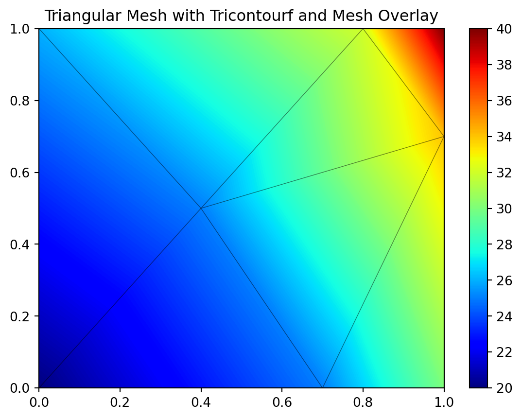
First, let us examine the rendering of the complex triangular mesh using tricontourf. This method prioritizes visual smoothness, effectively hiding the boundaries of the individual triangles by drawing a large number of filled contours.
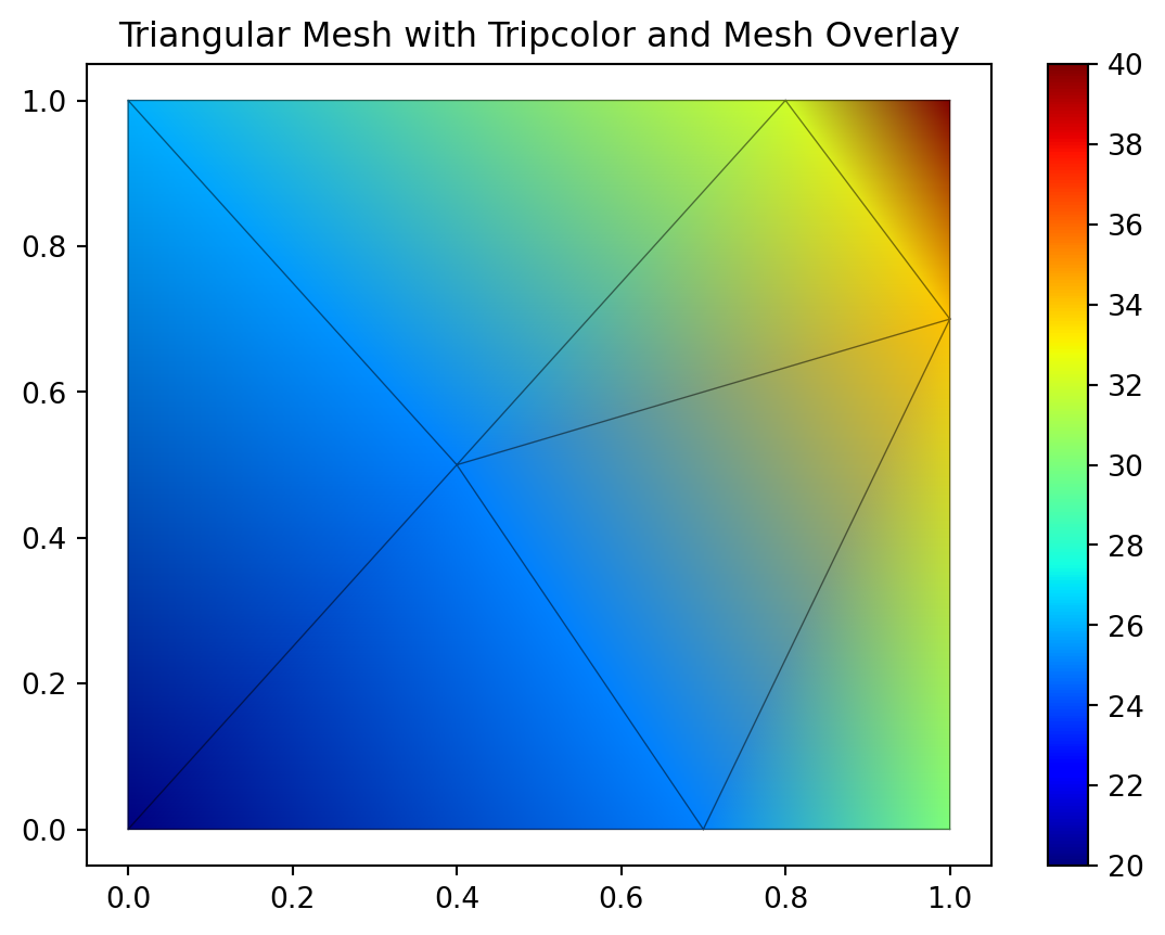
Now, let us consider the tripcolor rendering of the same complex mesh. This method is fundamentally different, directly rendering each triangle with linear color interpolation.
The tripcolor function with Gouraud shading offers high performance. Its primary advantage is efficiency, leveraging direct rendering pathways that are often hardware-accelerated. Its main disadvantage, however, arises from how it maps data to color. tripcolor performs a mathematically linear interpolation on the data values between vertices, and only then maps the resulting value to a color. If the colormap itself does not have a perceptually uniform gradient (and most, like ‘jet’, do not), the final plot will not visually reproduce the color transitions seen in the colorbar. This was the issue we observed in the initial quadrilateral example. For applications where faithfully representing the colormap’s specific gradient is visually critical, tripcolor can be inadequate.
In contrast, tricontourf achieves superior visual smoothness, creating high-fidelity results that are less sensitive to the underlying triangulation. This comes at a computational cost, as its multi-step process of gridding, interpolating, and drawing many contour polygons is computationally intensive and scales with the number of levels specified.
Given these characteristics, we can establish clear selection criteria. For large pre-triangulated meshes from finite element analysis, tripcolor is typically the appropriate choice since performance is critical and the individual elements are usually small enough that interpolation artifacts are not visually distracting. Conversely, when generating high-quality figures of a few large polygons for exercises or instructional materials, tricontourf is often the superior method. The performance penalty is acceptable in this context, and the resulting visual smoothness more accurately conveys the continuous nature of the underlying data field, free of triangulation artifacts.
Generating Smoother Gradients by Subdivision
We have established a trade-off between the direct, performant rendering of tripcolor and the visually smooth but computationally expensive approach of tricontourf. There is, however, a third strategy: we can manually refine our mesh before plotting. By subdividing each triangle into smaller triangles and interpolating the data to the new vertices, we create a higher-resolution mesh. When this refined mesh is rendered with the fast tripcolor function, the result appears smooth because the individual linear interpolations occur over much smaller areas. This approach moves the complexity from the rendering stage to a data pre-processing stage.
Let us begin with a simple unit square, defined by four vertices and two triangles, with a temperature value at each vertex.
We can now write a loop to iteratively subdivide this mesh. In each iteration, we will iterate over every triangle, find the midpoint of each of its three edges, and replace the original triangle with four smaller ones. The temperature values for the new midpoint vertices are linearly interpolated from their parent vertices.
The following code performs four such subdivisions and plots the state of the mesh at each stage, demonstrating how the grid becomes finer and the tripcolor plot becomes smoother.
Code
def subdivide(nodes, temps, triangles):""" Performs one level of subdivision on a triangular mesh. Each triangle is split into four smaller triangles. """ new_triangles = []# Use lists for dynamic appending, convert to numpy array at the end new_nodes =list(nodes) new_temps =list(temps) midpoint_cache = {}def get_or_create_midpoint(u_idx, v_idx): edge_key =tuple(sorted((u_idx, v_idx)))if edge_key in midpoint_cache:return midpoint_cache[edge_key]# Create new midpoint mid_point_coords = (new_nodes[u_idx] + new_nodes[v_idx]) /2.0 mid_point_temp = (new_temps[u_idx] + new_temps[v_idx]) /2.0 new_nodes.append(mid_point_coords) new_temps.append(mid_point_temp) new_mid_point_idx =len(new_nodes) -1 midpoint_cache[edge_key] = new_mid_point_idxreturn new_mid_point_idxfor tri in triangles: v0_idx, v1_idx, v2_idx = tri m01_idx = get_or_create_midpoint(v0_idx, v1_idx) m12_idx = get_or_create_midpoint(v1_idx, v2_idx) m20_idx = get_or_create_midpoint(v2_idx, v0_idx) new_triangles.extend([ [v0_idx, m01_idx, m20_idx], [v1_idx, m12_idx, m01_idx], [v2_idx, m20_idx, m12_idx], [m01_idx, m12_idx, m20_idx] ])return np.array(new_nodes), np.array(new_temps), np.array(new_triangles)# Store meshes for plottingmeshes = []nodes, temps, triangles = P_initial, T_initial, connectivity_initialmeshes.append((nodes, temps, triangles))# Perform 7 subdivisionsfor _ inrange(7): nodes, temps, triangles = subdivide(nodes, temps, triangles) meshes.append((nodes, temps, triangles))# Plot the resultsfig, axes = plt.subplots(4, 2, figsize=(8, 12), sharex=True, sharey=True)axes_flat = axes.flatten()alpha0 =0.5for i, (nodes_i, temps_i, triangles_i) inenumerate(meshes): ax = axes_flat[i] triang = Triangulation(nodes_i[:, 0], nodes_i[:, 1], triangles_i) tpc = ax.tripcolor(triang, temps_i, cmap='jet', shading='gouraud', vmin=20, vmax=40) ax.triplot(triang, 'k-', lw=1, alpha=alpha0/(i+1)) ax.set_title(f"Subdivision Level {i}\n{len(nodes_i)} nodes, {len(triangles_i)} tris") ax.set_aspect('equal')fig.tight_layout()plt.show()
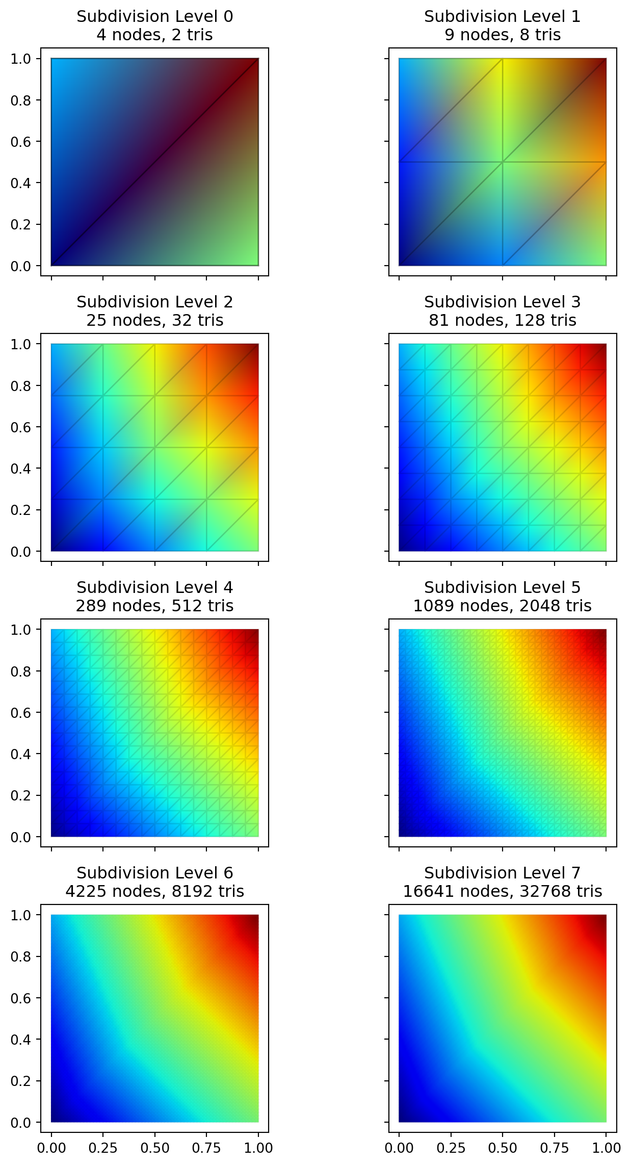
Iterative mesh refinement. The initial mesh (level 0) and seven subsequent subdivisions. Each plot uses the performant tripcolor function, but the visual result becomes smoother as the underlying mesh resolution increases.
This manual refinement strategy provides another tool in our arsenal. It grants explicit, data-level control over the resolution of the final plot, ensuring that even a performant, linear rendering engine like tripcolor can produce visually smooth results. The primary trade-off is the increased complexity of the pre-processing code and the higher memory footprint required to store the refined mesh data.
Performance Comparison: Subdivision vs. tricontourf Levels
We have discussed the conceptual trade-offs between two methods for achieving a visually smooth plot: manually increasing mesh resolution for tripcolor, and increasing the number of contour levels for tricontourf. We will now quantitatively compare the performance of these two strategies.
The following code measures the time required for each approach. For the subdivision method, we time 8 successive refinements. For the tricontourf method, we time its execution on the original coarse mesh while doubling the number of levels for 8 steps (from 1 to 256).
Code
import timeimport numpy as npimport matplotlib.pyplot as pltfrom matplotlib.tri import Triangulationdef subdivide(nodes, triangles):"""Subdivides a mesh without recalculating temperatures for performance test.""" new_triangles = [] new_nodes =list(nodes) midpoint_cache = {}def get_or_create_midpoint(u_idx, v_idx): edge_key =tuple(sorted((u_idx, v_idx)))if edge_key in midpoint_cache:return midpoint_cache[edge_key] mid_point_coords = (new_nodes[u_idx] + new_nodes[v_idx]) /2.0 new_nodes.append(mid_point_coords) new_mid_point_idx =len(new_nodes) -1 midpoint_cache[edge_key] = new_mid_point_idxreturn new_mid_point_idxfor tri in triangles: v0_idx, v1_idx, v2_idx = tri m01_idx = get_or_create_midpoint(v0_idx, v1_idx) m12_idx = get_or_create_midpoint(v1_idx, v2_idx) m20_idx = get_or_create_midpoint(v2_idx, v0_idx) new_triangles.extend([ [v0_idx, m01_idx, m20_idx], [v1_idx, m12_idx, m01_idx], [v2_idx, m20_idx, m12_idx], [m01_idx, m12_idx, m20_idx] ])return np.array(new_nodes), np.array(new_triangles)# --- Timing for Subdivision + tripcolor ---subdivision_times = []n_triangles = []nodes = np.array([[0., 0.], [1., 0.], [1., 1.], [0., 1.]])triangles = np.array([[0, 1, 2], [0, 2, 3]])for i inrange(9): # 0 (initial) + 8 subdivisions# Re-generate temps array based on current number of nodes# In a real scenario this would be interpolated, but for a performance# test we can generate random data of the correct size. temps = np.random.rand(len(nodes)) start_time = time.perf_counter() fig, ax = plt.subplots() triang = Triangulation(nodes[:, 0], nodes[:, 1], triangles) ax.tripcolor(triang, temps, cmap='jet', shading='gouraud') fig.canvas.draw() # Force render end_time = time.perf_counter() plt.close(fig) # Close figure to save memory subdivision_times.append(end_time - start_time) n_triangles.append(len(triangles))if i <8: # Don't subdivide on the last iteration nodes, triangles = subdivide(nodes, triangles)# --- Timing for tricontourf ---tricontourf_times = []levels_list = [2**i for i inrange(9)] # 1, 2, 4, ..., 256# Use the original coarse meshP_initial = np.array([[0., 0.], [1., 0.], [1., 1.], [0., 1.]])T_initial = np.array([20., 30., 40., 26.])triang_initial = Triangulation(P_initial[:, 0], P_initial[:, 1], np.array([[0, 1, 2], [0, 2, 3]]))for levels in levels_list: start_time = time.perf_counter() fig, ax = plt.subplots() ax.tricontourf(triang_initial, T_initial, levels=levels, cmap='jet') fig.canvas.draw() # Force render end_time = time.perf_counter() plt.close(fig) # Close figure to save memory tricontourf_times.append(end_time - start_time)# --- Plotting the Performance Comparison ---fig, ax = plt.subplots(figsize=(6, 4))iterations =range(9)ax.plot(iterations, subdivision_times, 'o-', label=f'Subdivision + tripcolor')ax.plot(iterations, tricontourf_times, 's-', label=f'tricontourf')ax.set_yscale('log')ax.set_xlabel('Refinement Iteration')ax.set_ylabel('Time (seconds, log scale)')ax.set_title('Performance Comparison: Subdivision vs. tricontourf Levels')ax.legend()ax.grid(True, which="both", ls="--")# Annotate x-axis with secondary labelsax2 = ax.twiny()ax2.set_xlabel("Number of Triangles (Subdivision) / Contour Levels (tricontourf)")ax2.set_xlim(ax.get_xlim())ax2.set_xticks(iterations)ax2.set_xticklabels([f"{n_tri}\n{lvl}"for n_tri, lvl inzip(n_triangles, levels_list)])fig.tight_layout()plt.show()
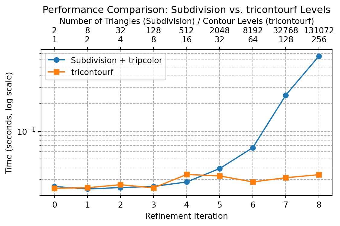
Performance comparison between manual mesh subdivision with tripcolor and increasing contour levels with tricontourf. Note the logarithmic scale on the time axis.
Visual Comparison of Refined Solutions
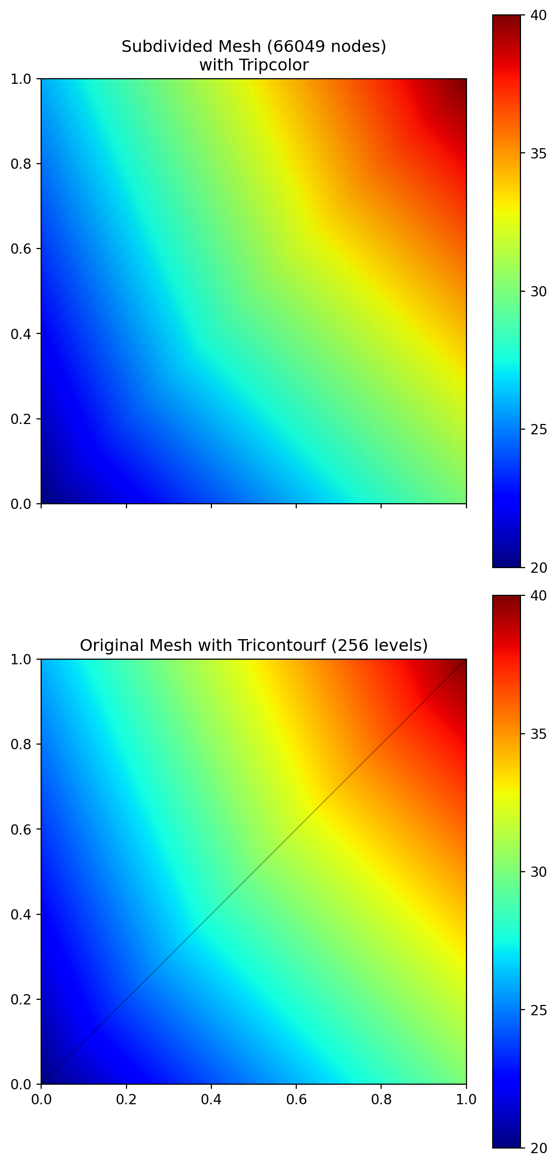
Finally, let us visually compare the refined solution obtained through mesh subdivision with tripcolor against the tricontourf method on the original coarse mesh. This side-by-side comparison demonstrates that both approaches can yield visually similar smooth gradients, albeit through different underlying mechanisms.
Code
# --- Visual Comparison of Refined Solutions ---import numpy as npimport matplotlib.pyplot as pltfrom matplotlib.tri import Triangulation, LinearTriInterpolator# Redefine the full subdivide function for this block to be self-containeddef subdivide(nodes, temps, triangles):""" Performs one level of subdivision on a triangular mesh. Each triangle is split into four smaller triangles. """ new_triangles = [] new_nodes =list(nodes) new_temps =list(temps) midpoint_cache = {}def get_or_create_midpoint(u_idx, v_idx): edge_key =tuple(sorted((u_idx, v_idx)))if edge_key in midpoint_cache:return midpoint_cache[edge_key] mid_point_coords = (new_nodes[u_idx] + new_nodes[v_idx]) /2.0 mid_point_temp = (new_temps[u_idx] + new_temps[v_idx]) /2.0 new_nodes.append(mid_point_coords) new_temps.append(mid_point_temp) new_mid_point_idx =len(new_nodes) -1 midpoint_cache[edge_key] = new_mid_point_idxreturn new_mid_point_idxfor tri in triangles: v0_idx, v1_idx, v2_idx = tri m01_idx = get_or_create_midpoint(v0_idx, v1_idx) m12_idx = get_or_create_midpoint(v1_idx, v2_idx) m20_idx = get_or_create_midpoint(v2_idx, v0_idx) new_triangles.extend([ [v0_idx, m01_idx, m20_idx], [v1_idx, m12_idx, m01_idx], [v2_idx, m20_idx, m12_idx], [m01_idx, m12_idx, m20_idx] ])return np.array(new_nodes), np.array(new_temps), np.array(new_triangles)# Unit square dataP_initial = np.array([[0., 0.], [1., 0.], [1., 1.], [0., 1.]])T_initial = np.array([20., 30., 40., 26.])connectivity_initial = np.array([[0, 1, 2], [0, 2, 3]])# --- Subdivision solution (8 levels of subdivision) ---nodes_sub, temps_sub, triangles_sub = P_initial, T_initial, connectivity_initialfor _ inrange(8): # Perform 8 subdivisions nodes_sub, temps_sub, triangles_sub = subdivide(nodes_sub, temps_sub, triangles_sub)# --- tricontourf solution (256 levels) ---triang_coarse = Triangulation(P_initial[:, 0], P_initial[:, 1], connectivity_initial)# --- Plotting side-by-side ---fig, axes = plt.subplots(2, 1, figsize=(6, 12), sharex=True, sharey=True)# Plot 1: Subdivided + tripcolorax0 = axes[0]triang_sub = Triangulation(nodes_sub[:, 0], nodes_sub[:, 1], triangles_sub)tpc = ax0.tripcolor(triang_sub, temps_sub, cmap='jet', shading='gouraud', vmin=T_initial.min(), vmax=T_initial.max())ax0.triplot(triang_sub, 'k-', lw=0.1, alpha=0.1) # Show very faint meshax0.set_title(f"Subdivided Mesh ({len(nodes_sub)} nodes)\nwith Tripcolor")ax0.set_aspect('equal')fig.colorbar(tpc, ax=ax0, ticks=np.arange(20, 41, 5))# Plot 2: tricontourf on coarse meshax1 = axes[1]levels_tc = np.linspace(T_initial.min(), T_initial.max(), 256)cf = ax1.tricontourf(triang_coarse, T_initial, levels=levels_tc, cmap='jet')ax1.triplot(triang_coarse, 'k-', lw=0.5, alpha=0.5) # Show original coarse meshax1.set_title(f"Original Mesh with Tricontourf (256 levels)")ax1.set_aspect('equal')fig.colorbar(cf, ax=ax1, ticks=np.arange(20, 41, 5))fig.tight_layout()plt.show()
MechanicsKit.Patch Examples
The MechanicsKit library provides a MATLAB-like patch function that automatically handles the trade-offs discussed in this document. The function automatically selects between tricontourf and tripcolor based on mesh size and colormap characteristics, providing optimal visual quality and performance without requiring manual intervention.
Automatic Method Selection
The patch function implements automatic method selection when FaceColor='interp' is specified. For small meshes with fewer than 100 elements using non-linear colormaps such as ‘jet’, ‘hsv’, or ‘hot’, the function selects tricontourf with 256 levels to achieve high visual fidelity. For large meshes or when using perceptually uniform colormaps such as ‘viridis’ or ‘plasma’, the function selects tripcolor with Gouraud shading to prioritize performance. Users can override this automatic selection using the interpolation_method parameter to force either approach when specific requirements demand explicit control.
Example: Single Quadrilateral with Different Colormaps
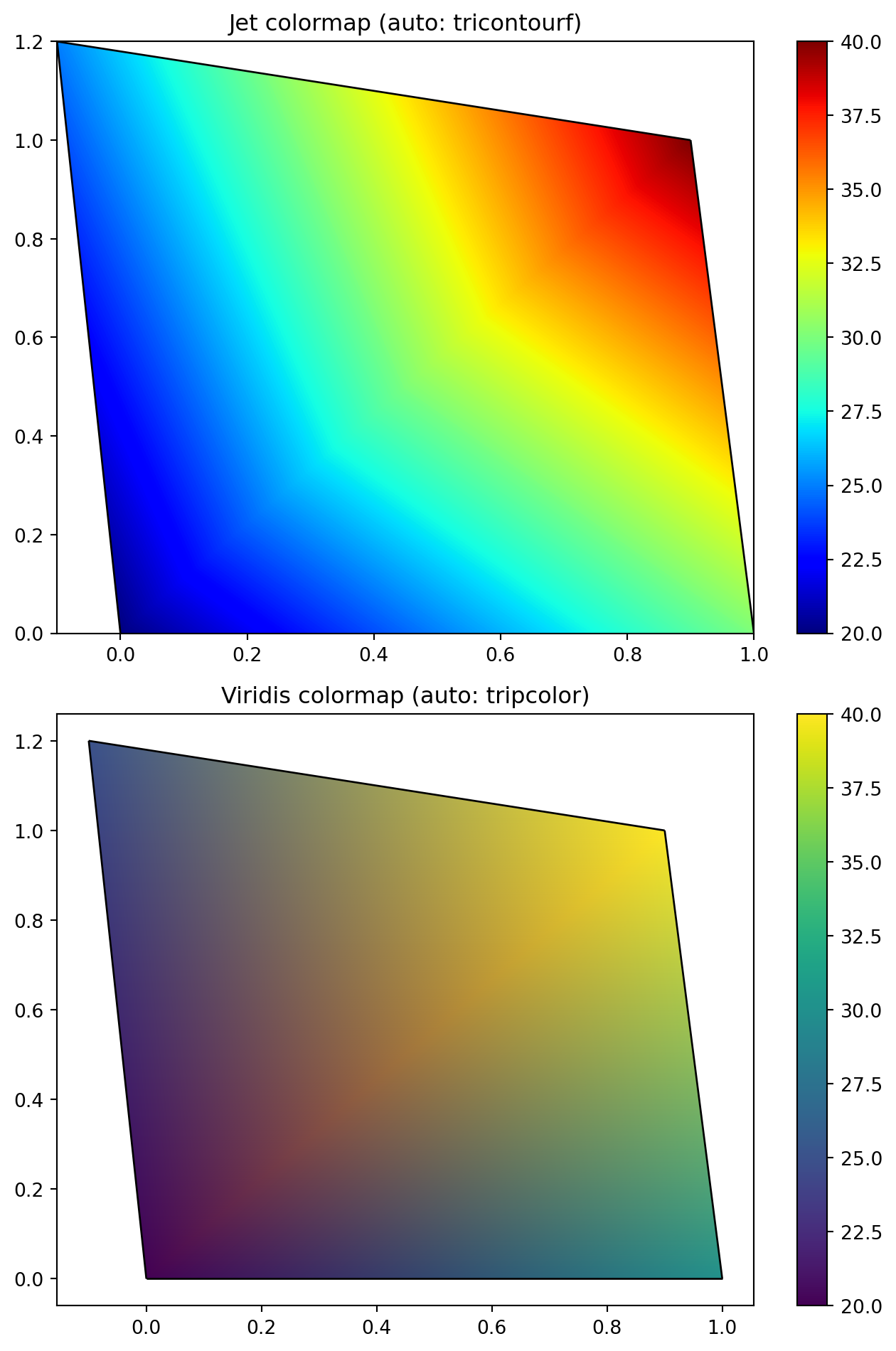
Let us replicate the MATLAB example from the introduction using the MechanicsKit patch function:
Notice how the automatic selection provides optimal results for both cases: smooth, accurate colors for the jet colormap using tricontourf, and efficient rendering for the perceptually uniform viridis colormap using tripcolor.
Example: Comparing Interpolation Methods
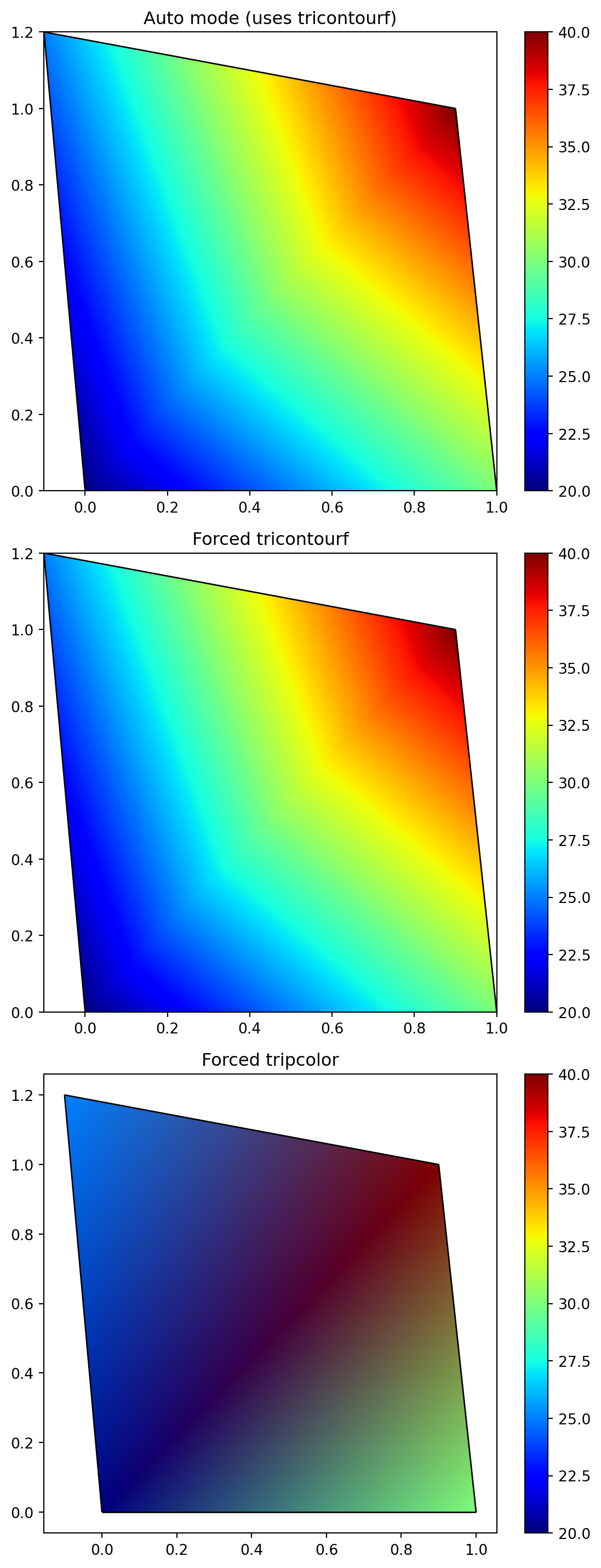
The interpolation_method parameter allows explicit control over the rendering method:
The visual difference is clear: tricontourf (upper and middle) produces vibrant, accurate color gradients that match the colorbar, while tripcolor (lower) shows the RGB interpolation artifacts discussed earlier in this document, resulting in muddier, less accurate colors.
Example: Complex Triangular Mesh
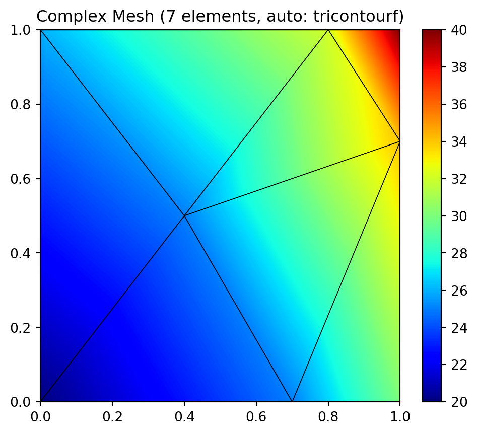
For the complex triangular mesh example, the automatic selection provides excellent results:
With only 7 elements and a non-linear colormap, the automatic mode correctly selects tricontourf, producing a smooth, high-quality visualization suitable for publication or instructional materials.