Code
import matplotlib.pyplot as plt
import numpy as np
import sympy as sp
from mechanicskit import fplot
plt.style.use('seaborn-v0_8-whitegrid')
plt.rcParams['figure.dpi'] = 200When we are faced with the task of evaluating a definite integral. We may want to do this analytically, i.e., by finding an antiderivative and evaluating it at the boundaries. However, this is not always possible. Furthermore, even if we can find an antiderivative, it may be computationally expensive to evaluate it. We might try to create an intragration rule which is easy to evaluate.
Let’s say, we want to integrate some function \(f(x)\)
\[ \int_a^b f(x) d x \]
We are immediately faced with how to handle the general limits of integration \(a\) and \(b\). The limits need to be handled in a way that is independent of the integration rule we choose. A common way to do this is to map the limits of integration to a standard range, e.g., \([0,1]\) or \([-1,1]\).
We can take any range \(x \in[a, b]\) and map it to the range \(\xi \in[0,1]\) using iso-parametric mapping: \(x(\xi):=(1-\xi) a+\xi b\) and its derivative (or map) \(\frac{d x}{d \xi}=b-a\) then we have
\[ \boxed{\int_a^b f(x) d x=\int_0^1 f(x(\xi)) \frac{d x}{d \xi} d \xi=(b-a) \int_0^1 f(x(\xi)) d \xi} \]
Example:
Let’s say we want to integrate some polynomial of order \(n\)
\[ \int_a^b x^n d x=(b-a) \int_0^1 x(\xi)^n d \xi=(b-a) \int_0^1((1-\xi) a+\xi b)^n d \xi=-\frac{a^{n+1}-b^{n+1}}{n+1} \]
Giving us a rule for integrating polynomials of order \(n\) over any range \([a,b]\), which can be implemented in computer code as a lookup table for fast evaluation. Ok, so this can be used to integrate e.g.,
\[ \int_2^5 2 x-4 x^2 d x=-2 \frac{a^{1+1}-b^{1+1}}{1+1}--4 \frac{a^{2+1}-b^{2+1}}{2+1}=-135 \]
But in general it is awkward to use this rule to integrate e.g., \(\int_{x_1}^{x_2}(1-x)(1-x) d x\) or \(\int_{x_1}^{x_2} \varphi^T \varphi d x\) without additional preparation which makes it cumbersome to implement in a computer program and run efficiently.
The same goes for the integration rulse such as
\[ \int_{-1}^1 x^n d x= \begin{cases}\frac{2}{n+1} & \text { if } n \text { is even } \\ 0 & \text { if } n \text { is odd }\end{cases} \]
and
\[ \int_0^1 x^n d x=\frac{1}{n+1} \]
We want a more general approach to numerical integration
Let’s consider a polynomial function \(f(x)=1+3 x^2-x^3\) for \(x \in[0,3]\)
import matplotlib.pyplot as plt
import numpy as np
import sympy as sp
from mechanicskit import fplot
plt.style.use('seaborn-v0_8-whitegrid')
plt.rcParams['figure.dpi'] = 200x = sp.Symbol('x')
f_expr = 1 + 3*x**2 - x**3
x1 = 0
x2 = 3fig, ax = plt.subplots(figsize=(8, 5))
fplot(f_expr, range=(x1, x2), color='blue', linewidth=2,
label=f'$f(x) = {sp.latex(f_expr)}$')
f_numeric = sp.lambdify(x, f_expr, 'numpy')
x_fill = np.linspace(x1, x2, 500)
y_fill = f_numeric(x_fill)
ax.fill_between(x_fill, y_fill, color='lightblue', alpha=0.5, label=f'Area from {x1} to {x2}')
ax.set_xlabel('$x$')
ax.set_ylabel('$f(x)$')
ax.set_title('Plot of $f(x)$ and Shaded Integral Area')
ax.axhline(0, color='black', linewidth=0.5) # Add x-axis
ax.axvline(0, color='black', linewidth=0.5) # Add y-axis
ax.grid(True, linestyle='--', alpha=0.7)
ax.legend(loc='upper left')
ax.set_xlim(x1, x2)
ax.set_ylim(0, max(y_fill)*1.1)
plt.show()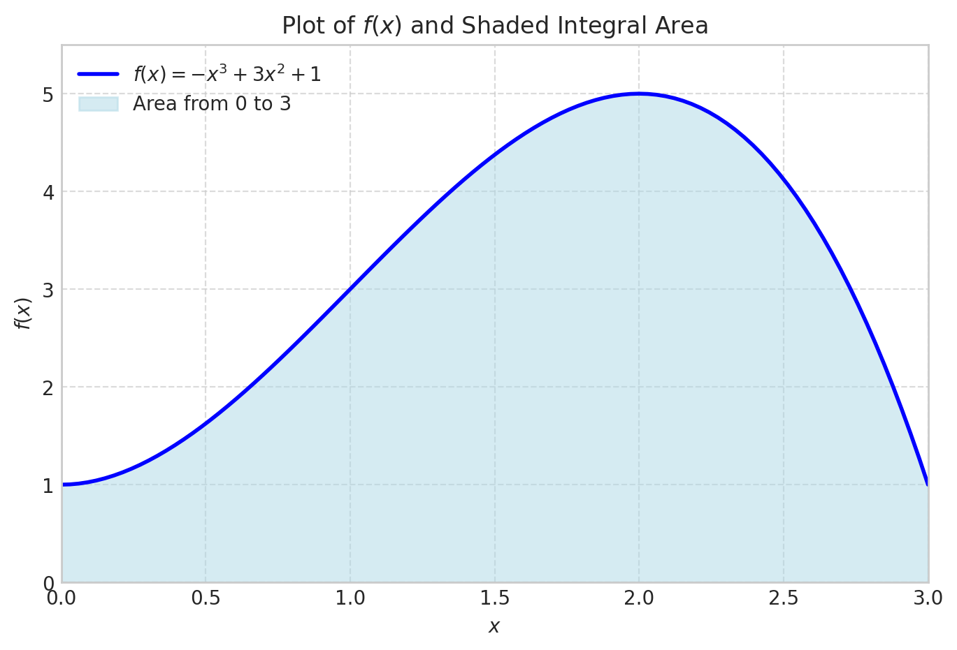
We can integrate this analytically
integral_value = sp.integrate(f_expr, (x, x1, x2))
integral_value\(\displaystyle \frac{39}{4}\)
integral_value.evalf()\(\displaystyle 9.75\)
This works very well even for function that do not have simple symbolic integrals.
f_expr = 1/sp.sqrt(sp.sin(x))
x1 = 0
x2 = 1fig, ax = plt.subplots(figsize=(8, 5))
x1 = 0.01
fplot(f_expr, range=(x1, x2), color='blue', linewidth=2,
label=f'$f(x) = {sp.latex(f_expr)}$')
f_numeric = sp.lambdify(x, f_expr, 'numpy')
x_fill = np.linspace(x1, x2, 500)
y_fill = f_numeric(x_fill)
ax.fill_between(x_fill, y_fill, color='lightblue', alpha=0.5, label=f'Area from {x1} to {x2}')
ax.set_xlim(x1, x2)
ax.set_ylim(0, max(y_fill)*1.1)
ax.legend(loc='upper right')
ax.grid(False)
plt.show()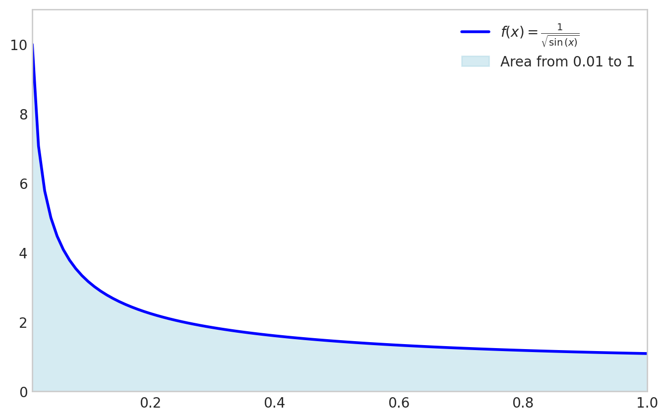
sp.integrate(f_expr, (x, x1, x2))\(\displaystyle \int\limits_{0.01}^{1} \frac{1}{\sqrt{\sin{\left(x \right)}}}\, dx\)
x1 = 0
sp.integrate(f_expr, (x, x1, x2)).evalf()\(\displaystyle 2.03480531920757\)
Another example is the function \(f(x)=e^{\cos(x)}\) for \(x \in[0,3]\)
f_expr = sp.exp(sp.cos(x))
x1 = 0; x2 = 1fig, ax = plt.subplots(figsize=(8, 5))
fplot(f_expr, range=(x1, x2), color='blue', linewidth=2,
label=f'$f(x) = {sp.latex(f_expr)}$')
f_numeric = sp.lambdify(x, f_expr, 'numpy')
x_fill = np.linspace(x1, x2, 500)
y_fill = f_numeric(x_fill)
ax.fill_between(x_fill, y_fill, color='lightblue', alpha=0.5, label=f'Area from {x1} to {x2}')
ax.set_xlim(x1, x2)
ax.set_ylim(0, max(y_fill)*1.1)
ax.legend(loc='upper right')
ax.grid(False)
plt.show()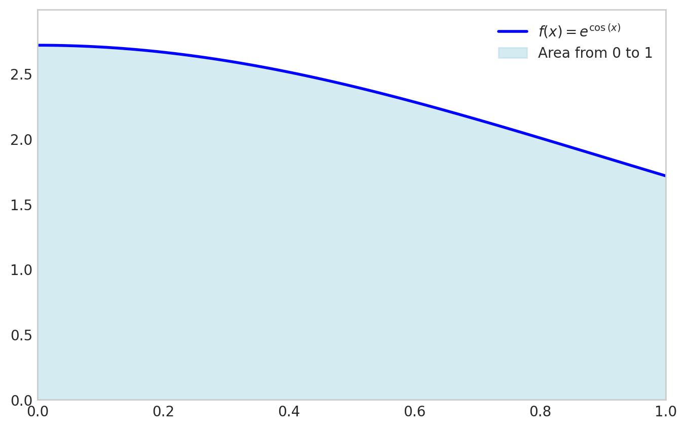
sp.integrate(f_expr, (x, x1, x2))\(\displaystyle \int\limits_{0}^{1} e^{\cos{\left(x \right)}}\, dx\)
There are two options here:
sp.integrate(f,(x, x1, x2)).evalf()sympy.Integral(f,(x, x1, x2)).evalf()sp.integrate(f_expr, (x, 0, 1)).evalf()\(\displaystyle 2.34157484171305\)
sp.Integral(f_expr, (x, 0, 1)).evalf()\(\displaystyle 2.34157484171305\)
The outcome is the same, but the second option is often faster since it does not try to find a symbolic expression for the integral. If sp.integral fails it will fall back to sp.Integral. Relying on this fallback is not good practice.
For reliably computing the numerical value of an integral, always use sympy.Integral(...).evalf(). It is the direct, explicit, and robust method.
Use sympy.integrate() only when you need the symbolic antiderivative itself.
Now, let’s go back to basics and take a look at the Riemann sum.
\[ \int_a^b f(x) \approx \frac{b-a}{N} \sum_{i=1}^N f\left(x_i\right) \]
x = sp.Symbol('x')
f_expr = 1 + 3*x**2 - x**3
x1 = 0; x2 = 3
from matplotlib.animation import FuncAnimation
from IPython.display import HTML
import matplotlib
matplotlib.rcParams['animation.embed_limit'] = 50 # Increase if needed
from matplotlib.colors import to_rgba
# Define N values
N_values = [1, 2, 3, 4, 5, 10, 20, 30, 40, 50, 100, 150, 200]
N_values = list(range(2, 20, 1)) + list(range(20, 201, 5))
def animate(frame_idx):
"""Animation function for each frame"""
ax.clear()
N = N_values[frame_idx]
# Compute Riemann sum data
f_numeric = sp.lambdify(x, f_expr, 'numpy')
dx = (x2 - x1) / N
x_points = np.linspace(x1 + dx/2, x2 - dx/2, N) # Center points for bars
y_points = f_numeric(x_points - dx/2) # Left Riemann sum (use left edge)
riemann_sum = dx * np.sum(y_points)
# Compute exact integral
exact_integral = sp.Integral(f_expr, (x, x1, x2)).evalf()
error = abs(float(exact_integral) - riemann_sum)
# Determine edge opacity based on N
if N <= 10:
edge_alpha = 0.5
edge_color = to_rgba('black', alpha=edge_alpha)
linewidth = 1
elif N < 75:
edge_alpha = 0.5 - ((N - 10) / (75 - 10))*0.5
edge_color = to_rgba('black', alpha=edge_alpha)
linewidth = 1
else:
edge_color = 'lightcoral'
# edge_color = to_rgba('black', alpha=0)
linewidth = 1
# Plot Riemann sum as bars
ax.bar(x_points, y_points, width=dx, align='center',
facecolor='lightcoral',
# alpha=1,
edgecolor=edge_color, linewidth=linewidth,
label='Riemann Sum')
# Plot the function on top
x_plot = np.linspace(x1, x2, 500)
y_plot = f_numeric(x_plot)
ax.plot(x_plot, y_plot, color='blue', linewidth=2,
label=f'$f(x) = {sp.latex(f_expr)}$', zorder=5)
# Set labels and limits
ax.set_xlabel('$x$', fontsize=12)
ax.set_ylabel('$f(x)$', fontsize=12)
ax.set_xlim(x1, x2)
y_max = max(f_numeric(np.linspace(x1, x2, 500)))
ax.set_ylim(0, y_max * 1.2)
ax.grid(True, linestyle='--', alpha=0.7)
ax.axhline(0, color='black', linewidth=0.5)
ax.axvline(0, color='black', linewidth=0.5)
# Add text box with results
textstr = f'$N = {N}$\n'
textstr += f'Exact Integral: ${exact_integral:.6f}$\n'
textstr += f'Riemann Sum: ${riemann_sum:.6f}$\n'
textstr += f'Error: ${error:.6f}$'
props = dict(boxstyle='round', facecolor='wheat', alpha=0.8)
ax.text(0.02, 0.98, textstr, transform=ax.transAxes, fontsize=11,
verticalalignment='top', bbox=props)
ax.legend(loc='upper right')
# Create figure and axis (close to prevent static display)
fig, ax = plt.subplots(figsize=(6, 4))
plt.close(fig) # Prevent static image from showing
# Create animation
anim = FuncAnimation(fig, animate, frames=len(N_values),
interval=800, repeat=True)
# Display as interactive HTML
# HTML(anim.to_jshtml())
# Get the HTML and wrap it with responsive CSS
anim_html = anim.to_jshtml()
# Wrap with CSS to make it responsive and fit to 100% width
responsive_html = f"""
<div style="width: 100%; max-width: 100%; overflow: hidden;">
<style>
.animation-container {{
width: 100% !important;
max-width: 100% !important;
}}
.animation-container img {{
width: 100% !important;
height: auto !important;
}}
</style>
<div class="animation-container">
{anim_html}
</div>
</div>
"""
HTML(responsive_html)Let’s take a look at the error we’re making numerically
\[ \epsilon=\left|I_{\text {Riemann }}-I_{\text {exact }}\right| \]
N = 200
f_numeric = sp.lambdify(x, f_expr, 'numpy')
dx = (x2 - x1) / N
x_points = np.linspace(x1, x2, N)
y_points = f_numeric(x_points)
I_riemann = dx * np.sum(y_points)
I_exact = sp.Integral(f_expr, (x, x1, x2)).evalf()error_riemann = abs( I_exact - I_riemann)
error_riemann\(\displaystyle 0.03391959798995\)
Note that the absolute integration error is still significantly large after 200 function evaluations!
We can improve the accuracy of the numerical integration by using the trapezoidal rule
First we approximate \(f(x)\) linearly: \(f(x) \approx \varphi_1(x) f(a)+\varphi_2(x) f(b)=\frac{b-x}{b-a} f(a)+\frac{x-a}{b-a} f(b)\) then we have
\[ I \approx \frac{f(a)}{b-a} \int_a^b b-x d x+\frac{f(b)}{b-a} \int_a^b x-a d x=\frac{f(a)}{b-a}\left[b x-\frac{1}{2} x^2\right]_a^b+\frac{f(b)}{b-a}\left[\frac{1}{2} x^2-a x\right]_a^b \\ \]
$$ =(b^2- b^2-a b- a^2)+( b^2-a b- a2-a2) \
$$
\[ =\frac{f(a)}{b-a} \frac{1}{2}(b-a)^2+\frac{f(b)}{b-a} \frac{1}{2}(b-a)^2 \\ \]
\[ =\frac{1}{2}(b-a)(f(a)+f(b)) \]
This is called the trapezoidal rule. And for a chained approximation with \(N+1\) evenly spaced points the approximation becomes:
\[ \boxed{\int_a^b f(x) d x \approx \frac{b-a}{2 N} \sum_{i=1}^N\left(f\left(x_i\right)+f\left(x_{i+1}\right)\right)} \]
For example for the function above using \(N=200\) we have:
f_expr = 1 + 3*x**2 - x**3
x1 = 0; x2 = 3
I_exact = sp.Integral(f_expr, (x, x1, x2)).evalf()
N = 200
f_numeric = sp.lambdify(x, f_expr, 'numpy')
x_points = np.linspace(x1, x2, N+1)
x_i = x_points[0:-1]
x_i1 = x_points[1:]
I_trapz = np.sum(f_numeric(x_i) + f_numeric(x_i1)) * (x2-x1)/(2*N)
I_trapznp.float64(9.74983125)error_trapz = abs(I_exact - I_trapz)
error_trapz\(\displaystyle 0.000168750000000273\)
Trapezoidal rule gives much better accuracy than the Riemann sum for the same number of function evaluations! There is a built-in function in numpy for the trapezoidal rule: numpy.trapz
np.trapezoid(f_numeric(x_points), x_points)np.float64(9.74983125)error_riemann/error_trapz\(\displaystyle 201.005025125305\)
We see an 200x improvement in accuracy for the same number of function evaluations!
from matplotlib.animation import FuncAnimation
from IPython.display import HTML
import matplotlib
matplotlib.rcParams['animation.embed_limit'] = 50 # Increase if needed
from matplotlib.colors import to_rgba
f_expr = 1 + 3*x**2 - x**3
x1 = 0; x2 = 3
f_numeric = sp.lambdify(x, f_expr, 'numpy')
I_exact = sp.Integral(f_expr, (x, x1, x2)).evalf()
N_values = list(range(4, 20, 1)) + list(range(20, 201, 5))
# N_values = [4,8,15]
def makePlot(N):
x_points = np.linspace(x1, x2, N+1)
dx = (x2 - x1) / (N+1)
y_points = f_numeric(x_points)
I_riemann = dx * np.sum(y_points)
error_riemann = abs( I_exact - I_riemann)
x_i = x_points[0:-1]
x_i1 = x_points[1:]
I_trapz = np.sum(f_numeric(x_i) + f_numeric(x_i1)) * (x2-x1)/(2*N)
error_trapz = abs(I_exact - I_trapz)
if N <= 10:
edge_alpha = 0.5
edge_color = to_rgba('black', alpha=edge_alpha)
elif N < 50:
edge_alpha = 0.5 - ((N - 10) / (50 - 10))*0.5
edge_color = to_rgba('black', alpha=edge_alpha)
else:
edge_color = to_rgba('cyan', alpha=0)
# fig, ax = plt.subplots(figsize=(6, 4))
ax.grid(False)
for iel in range(N):
xs = [x_i[iel], x_i[iel], x_i1[iel], x_i1[iel]]
ys = [0, f_numeric(x_i[iel]), f_numeric(x_i1[iel]), 0]
ax.fill(xs, ys, facecolor = to_rgba('cyan', alpha=0.7),
edgecolor = edge_color)
# Plot the function on top
x_plot = np.linspace(x1, x2, 500)
y_plot = f_numeric(x_plot)
ax.plot(x_plot, y_plot, color='blue', linewidth=2,
label=f'$f(x) = {sp.latex(f_expr)}$', zorder=5)
# Set labels and limits
ax.set_xlabel('$x$', fontsize=12)
ax.set_ylabel('$f(x)$', fontsize=12)
ax.set_xlim(x1, x2)
y_max = max(f_numeric(np.linspace(x1, x2, 500)))
ax.set_ylim(0, y_max * 1.2)
ax.grid(True, linestyle='--', alpha=0.7)
ax.axhline(0, color='black', linewidth=0.5)
ax.axvline(0, color='black', linewidth=0.5)
# Add text box with results
textstr = f'$N = {N}$\n'
textstr += f'I_e: ${I_exact:.6f}$\n'
textstr += f'I_R: ${I_riemann:.6f}$, error:${error_riemann:.4f}$\n'
textstr += f'I_T: ${I_trapz:.6f}$, error:${error_trapz:.4f}$'
props = dict(boxstyle='round', facecolor='w', alpha=0.8)
ax.text(0.02, 0.98, textstr, transform=ax.transAxes, fontsize=10,
verticalalignment='top', bbox=props)
ax.legend(loc='upper right')
def animate(frame_idx):
"""Animation function for each frame"""
ax.clear()
N = N_values[frame_idx]
makePlot(N)
# Create figure and axis (close to prevent static display)
fig, ax = plt.subplots(figsize=(6, 4))
plt.close(fig) # Prevent static image from showing
# Create animation
anim = FuncAnimation(fig, animate, frames=len(N_values),
interval=800, repeat=True)
# Display as interactive HTML
# HTML(anim.to_jshtml())
# Get the HTML and wrap it with responsive CSS
anim_html = anim.to_jshtml()
# Wrap with CSS to make it responsive and fit to 100% width
responsive_html = f"""
<div style="width: 100%; max-width: 100%; overflow: hidden;">
<style>
.animation-container {{
width: 100% !important;
max-width: 100% !important;
}}
.animation-container img {{
width: 100% !important;
height: auto !important;
}}
</style>
<div class="animation-container">
{anim_html}
</div>
</div>
"""
HTML(responsive_html)The trapezoidal rule integrates linear polynomials exactly:
\[ \int_a^b p_1(x) d x = \frac{b-a}{2}(p_1(a)+p_1(b)) \]
x = sp.Symbol('x')
f_expr = 1 + 3*x
x1 = 0; x2 = 3
f_numeric = sp.lambdify(x, f_expr, 'numpy')
x_points = np.linspace(x1, x2, 2)
np.trapezoid(f_numeric(x_points), x_points)np.float64(16.5)sp.Integral(f_expr, (x, x1, x2)).evalf()\(\displaystyle 16.5\)
fig, ax = plt.subplots(figsize=(6, 4))
fplot(f_expr, range=(x1, x2), color='blue', linewidth=2,
label=f'$f(x) = {sp.latex(f_expr)}$')
x_fill = np.linspace(x1, x2, 2)
y_fill = f_numeric(x_fill)
ax.fill_between(x_fill, y_fill, color='lightblue', alpha=0.5, label=f'Area from {x1} to {x2}')
ax.grid(False)
ax.set_xlim(x1, x2)
ax.set_ylim(0, max(y_fill)*1.1)
fig.show()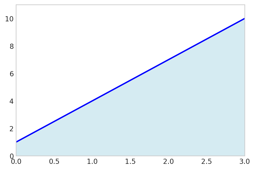
Since two points define a line, the trapezoidal rule will always give the exact result for linear polynomials.
But there is a cheaper way…
We can evaluate the midpoint \(\frac{a+b}{2}\) instead:
xm = (x1 + x2)/2
(x2-x1)*f_numeric(xm)16.5fig, ax = plt.subplots(figsize=(6, 4))
fplot(f_expr, range=(x1, x2), color='blue', linewidth=2,
label=f'$f(x) = {sp.latex(f_expr)}$')
x_fill = np.linspace(x1, x2, 2)
y_m = f_numeric(xm)
ax.fill_between(x_fill, [y_m], color='lightblue', alpha=0.5, label=f'Area from {x1} to {x2}')
ax.plot([xm], [y_m], color='k', marker='o')
ax.plot([x1, x2], [y_m, y_m], color='k', linestyle='-', lw=0.5)
ax.grid(False)
ax.set_xlim(x1, x2)
ax.set_ylim(0, 10)
fig.show()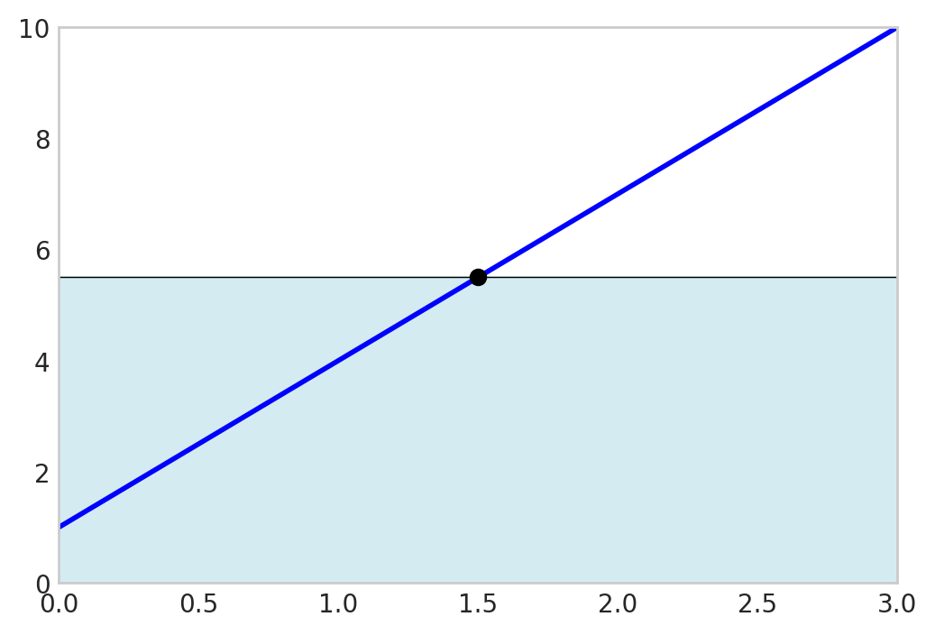
This is exact because the error above the graph cancels the error below the graph!
One rule to rule them all.
Gaussian quadrature is a powerful technique for numerical integration that offers a significant improvement in accuracy over simpler methods like the midpoint or trapezoidal rule. The idea behind Gaussian quadrature is to strategically choose the points at which the function is evaluated, rather than using equally spaced points. By selecting these optimal locations, known as nodes, and assigning specific weights to each, Gaussian quadrature can achieve exact results for polynomials up to a certain degree.
An n-point Gaussian quadrature rule can integrate a polynomial of degree 2n-1 exactly. This is a remarkable result and is what makes the method so powerful. For a given number of function evaluations, Gaussian quadrature provides the highest possible accuracy.
The general form of an n-point Gaussian quadrature for the standard domain \(x\in[-1,1]\) is:
\[ \boxed{\int_{-1}^{1} f(x) dx \approx \sum_{i=1}^{n} w_i f(x_i)} \]
where x_i are the nodes and w_i are the weights. Notice that the integral is defined on the interval [-1, 1]. This is the standard “reference” interval for Gaussian quadrature.
To use Gaussian quadrature on a different interval, say from \(a\) to \(b\), we need to perform a change of variables. We can map a new variable \(\xi\) in \([-1, 1]\) to our variable \(x\) in \([a, b]\) using the following linear transformation:
\[ x = \frac{b-a}{2}\xi + \frac{a+b}{2} \]
When we substitute this into the integral, we also need to change the differential \(dx\). We get the map by differentiating \(\frac{dx}{d\xi}\)
We have
\[ \int_a^b f(x) d x=\int_{-1}^1 f(x(\xi)) \frac{d x}{d \xi} d \xi \]
and with
\[ \dfrac{d x}{d \xi}=\frac{b-a}{2} \]
we get
\[ \int_{a}^{b} f(x) dx = \int_{-1}^{1} f\left(\frac{b-a}{2}\xi + \frac{a+b}{2}\right) \frac{b-a}{2} d\xi \]
Now, we can apply the Gaussian quadrature rule to the integral on the right-hand side.
The nodes, \(\xi_i\), are the roots of the \(n\)-th Legendre polynomial, \(P_n(\xi)\). The weights, \(w_i\), can then be calculated from these nodes. Below are the nodes and weights for integrating on the standard interval [-1, 1].
| \(n\) | Nodes (\(\xi_i\)) | Weights (\(w_i\)) |
|---|---|---|
| 1 | \(0\) | \(2\) |
| 2 | \(\pm 1/\sqrt{3} \approx \pm 0.57735\) | \(1\) |
| 3 | \(0\) \(\pm \sqrt{3/5} \approx \pm 0.77460\) |
\(8/9\) \(5/9\) |
| 4 | \(\pm \sqrt{ \frac{3 - 2\sqrt{6/5}}{7} } \approx \pm 0.33998\) \(\pm \sqrt{ \frac{3 + 2\sqrt{6/5}}{7} } \approx \pm 0.86114\) |
\(\frac{18 + \sqrt{30}}{36} \approx 0.65215\) \(\frac{18 - \sqrt{30}}{36} \approx 0.34785\) |
x = sp.Symbol('x')
f_expr = x
x1 = 0; x2 = 1
I_e = sp.Integral(f_expr, (x, x1, x2)).evalf()
I_e\(\displaystyle 0.5\)
gp = 0; gw = 2;
I_G = gw * f_expr.subs(x, (x2 - x1)/2 + x1) * (x2 - x1)/2
I_G\(\displaystyle 0.5\)
Ok, not a big deal, after all, even the Riemann sum is exact for linear polynomials.
How about a third order polynomial using only two function evaluations?
\[ \int_0^1 1+3 x-3 x^3 d x=\sum_i^2 p\left(x_i\right) \frac{1}{2}w_i\\ \]
where \(x_1=\frac{b-a}{2}\xi_1 + \frac{a+b}{2}\) and \(x_2=\frac{b-a}{2}\xi_2 + \frac{a+b}{2}\) and \(w_{1,2}=1\)
x = sp.Symbol('x')
p = lambda x: 1 + 3*x**2 - 3*x**3
sp.Integral(p(x), (x, 0, 1)).evalf()\(\displaystyle 1.25\)
a = 0; b = 1
gp = [-1/sp.sqrt(3), 1/sp.sqrt(3)]
gw = [1, 1]
x1 = gp[0]*(b - a)/2 + (b + a)/2
x2 = gp[1]*(b - a)/2 + (b + a)/2
dx = (b - a)/2
I_Gauss = p(x1)*gw[0]*dx + \
p(x2)*gw[1]*dx
I_Gauss\(\displaystyle - 1.5 \left(\frac{\sqrt{3}}{6} + 0.5\right)^{3} - 1.5 \left(0.5 - \frac{\sqrt{3}}{6}\right)^{3} + 1.5 \left(0.5 - \frac{\sqrt{3}}{6}\right)^{2} + 1.5 \left(\frac{\sqrt{3}}{6} + 0.5\right)^{2} + 1.0\)
I_Gauss.simplify()\(\displaystyle 1.25\)