8.3  Kinematics - Constraint Solving

import numpy as np
import matplotlib.pyplot as plt
import scipy
from matplotlib.animation import FuncAnimation
from IPython.display import HTML
import matplotlib
matplotlib.rcParams['animation.embed_limit'] = 60  # Increase if needed
from matplotlib.colors import to_rgba

r_OA = 100.0  # Length of link OA
r_CB = 75.0   # Length of link CB
rr_OC = np.array([250, 50])  
r_AB = np.sqrt((250 - 75)**2 + (100 - 50)**2)

def equations(vars, theta):
    """
    Args:
        vars: A list or tuple [phi, gamma] containing the angles
              of links OA and AB in radians.
    Returns:
        The distance between points B from A and B from C, this distance is zero for the correct set of phi and gamma.
    """
    phi, gamma = vars

    rr_OA = r_OA * np.array([np.sin(phi), np.cos(phi)]) 
    rr_AB = r_AB * np.array([np.sin(gamma), np.cos(gamma)])
    # Position of B calculated from chain O->A->B
    rr_OAB = rr_OA + rr_AB

    # Position of B calculated from chain C->B
    # [-sind(θ), cosd(θ)] which corresponds to an angle measured from the +y axis
    rr_CB = r_CB * np.array([-np.sin(theta), np.cos(theta)])
    rr_OCB = rr_OC + rr_CB

    return rr_OAB - rr_OCB

def is_valid_solution(theta, initial_guess, tolerance=1e-3):
    """Check if theta has a valid kinematic solution"""
    try:
        solution, info, ier, msg = scipy.optimize.fsolve(
            equations, initial_guess, args=(theta,), full_output=True
        )
        # Check if solver converged and residual is small
        residual = np.linalg.norm(info['fvec'])
        return ier == 1 and residual < tolerance, solution
    except:
        return False, None

# Find valid theta range by scanning
print("Finding valid theta range...")
theta_test = np.linspace(np.deg2rad(-30), np.deg2rad(300), 30+300)
thetas = []
initial_guess = np.deg2rad([50, 70])

for theta in theta_test:
    is_valid, sol = is_valid_solution(theta, initial_guess)
    if is_valid:
        thetas.append(theta)
        initial_guess = sol  # Use previous solution as next guess
        # print(f"Valid theta found: {np.rad2deg(theta):.1f}°")

if len(thetas) > 0:
    theta_min = thetas[0]
    theta_max = thetas[-1]
    print(f"Valid theta range: [{np.rad2deg(theta_min):.1f}°, {np.rad2deg(theta_max):.1f}°]")
    print(f"Number of valid configurations: {len(thetas)}")
else:
    print("No valid solutions found!")
    theta_min, theta_max = 0, 0

def plot_mechanism(rr_OA, rr_OB, rr_OC, theta):
    # Plot the links of the mechanism
    ax.plot(*zip([0,0], rr_OA), '-ko',lw=2)
    ax.plot(*zip(rr_OC, rr_OB), '-ko',lw=2)
    ax.plot(*zip(rr_OA, rr_OB), '-ko',lw=2)

    ax.text(rr_OA[0] + 5, rr_OA[1], 'A', fontsize=12)
    ax.text(rr_OB[0] + 5, rr_OB[1], 'B', fontsize=12)
    ax.text(rr_OC[0] + 5, rr_OC[1], 'C', fontsize=12)
    ax.text(5, 5, 'O', fontsize=12)
    ax.set_xlabel('x')
    ax.set_ylabel('y')
    ax.set_title(f'Three-Bar Linkage (θ = {np.rad2deg(theta):.1f}°)')
    ax.grid(True)
    ax.set_aspect('equal', adjustable='box') # Ensures correct proportions
    ax.set_xlim(-50, 300)
    ax.set_ylim(-50, 150)

# Only animate valid theta values
# thetas = np.linspace(theta_min, theta_max, 60)

fig, ax = plt.subplots(figsize=(10, 8))

def animate(frame_idx):
    """Animation function for each frame"""
    ax.clear()
    
    theta = thetas[frame_idx]
    initial_guess = np.deg2rad([50, 70]) 
    solution_rad = scipy.optimize.fsolve(equations, initial_guess, args=(theta,))
    phi_sol, gamma_sol = solution_rad

    rr_OA = r_OA * np.array([np.sin(phi_sol), np.cos(phi_sol)])
    rr_OB = rr_OA + r_AB * np.array([np.sin(gamma_sol), np.cos(gamma_sol)])

    plot_mechanism(rr_OA, rr_OB, rr_OC, theta)

# Create figure and axis (close to prevent static display)
plt.close(fig)  # Prevent static image from showing

# Create animation
anim = FuncAnimation(fig, animate, frames=len(thetas), 
                     interval=100, repeat=True)

# Get the HTML and wrap it with responsive CSS
anim_html = anim.to_jshtml()

# Wrap with CSS to make it responsive and fit to 100% width
responsive_html = f"""
<div style="width: 100%; max-width: 100%; overflow: hidden;">
    <style>
        .animation-container {{
            width: 100% !important;
            max-width: 100% !important;
        }}
        .animation-container img {{
            width: 100% !important;
            height: auto !important;
        }}
    </style>
    <div class="animation-container">
        {anim_html}
    </div>
</div>
"""
HTML(responsive_html)

# video_html = anim.to_html5_video()
# video_html = video_html.replace('controls', 'controls autoplay loop muted')
# video_html = video_html.replace(
#     '<video ', 
#     '<video style="width: 100%; height: auto;" '
# )
# HTML(video_html)

import numpy as np
import matplotlib.pyplot as plt
import scipy.optimize

import warnings
warnings.filterwarnings('ignore', message='The iteration is not making good progress')

# Mechanism parameters (same as geometric solution)
r = 50.0   # Crank length
L = 150.0  # Connecting rod length

def constraint_equations(vars, theta):
    """
    Constraint equations for crank-slider mechanism.
    
    Args:
        vars: [phi, x_A] - angle of connecting rod and slider position
        theta: crank angle (input)
        
    Returns:
        residuals: [eq1, eq2] - constraint equation residuals
    """
    phi, x_A = vars
    
    # Position of B (end of crank)
    rr_OB = r * np.array([-np.cos(theta), np.sin(theta)])
    
    # Position of A from B using connecting rod
    rr_BA = L * np.array([np.cos(phi), np.sin(phi)])
    
    # Position of A (computed from chain O->B->A)
    rr_OA_computed = rr_OB + rr_BA
    
    # Position of A (constrained to horizontal axis)
    rr_OA_constraint = np.array([x_A, 0])
    
    # Residuals (should be zero when constraints are satisfied)
    residuals = rr_OA_computed - rr_OA_constraint
    
    return residuals

# Solve for one configuration
theta_test = np.deg2rad(45)  # Test angle
initial_guess = [np.deg2rad(180), -150]  # Initial guess for [phi, x_A]

solution = scipy.optimize.fsolve(constraint_equations, initial_guess, args=(theta_test,))
phi_sol, x_A_sol = solution

print(f"For θ = {np.rad2deg(theta_test):.1f}°:")
print(f"  φ = {np.rad2deg(phi_sol):.2f}°")
print(f"  x_A = {x_A_sol:.2f} mm")

# Verify the solution
rr_OB = r * np.array([-np.cos(theta_test), np.sin(theta_test)])
rr_OA = np.array([x_A_sol, 0])
rr_BA = rr_OA - rr_OB
print(f"  |BA| = {np.linalg.norm(rr_BA):.2f} mm (should be {L:.2f} mm)")
print(f"  Residual: {np.linalg.norm(constraint_equations(solution, theta_test)):.2e}")

# Solve for full rotation
theta_range = np.linspace(0, 2*np.pi, 100)
phi_solutions = []
x_A_solutions = []

initial_guess = [np.deg2rad(180), -150]  # Start from a reasonable configuration

for theta in theta_range:
    try:
        sol = scipy.optimize.fsolve(constraint_equations, initial_guess, args=(theta,))
        phi_sol, x_A_sol = sol
        
        # Verify solution quality
        residual = np.linalg.norm(constraint_equations(sol, theta))
        if residual < 1e-6:  # Good solution
            phi_solutions.append(phi_sol)
            x_A_solutions.append(x_A_sol)
            initial_guess = sol  # Use previous solution as initial guess
        else:
            phi_solutions.append(np.nan)
            x_A_solutions.append(np.nan)
    except:
        phi_solutions.append(np.nan)
        x_A_solutions.append(np.nan)

phi_solutions = np.array(phi_solutions)
x_A_solutions = np.array(x_A_solutions)

# Plot results
fig, axes = plt.subplots(2, 1, figsize=(10, 8))

# Plot slider position
axes[0].plot(np.rad2deg(theta_range), x_A_solutions, 'b-', linewidth=2)
axes[0].set_xlabel('Crank angle θ [deg]')
axes[0].set_ylabel('Slider position $x_A$ [mm]')
axes[0].set_title('Slider Position vs Crank Angle')
axes[0].grid(True)

# Plot connecting rod angle
axes[1].plot(np.rad2deg(theta_range), np.rad2deg(phi_solutions), 'r-', linewidth=2)
axes[1].set_xlabel('Crank angle θ [deg]')
axes[1].set_ylabel('Connecting rod angle φ [deg]')
axes[1].set_title('Connecting Rod Angle vs Crank Angle')
axes[1].grid(True)

plt.tight_layout()
plt.show()

# Animation of crank-slider mechanism using constraint-based solution
import warnings
warnings.filterwarnings('ignore', message='The iteration is not making good progress')

from matplotlib.animation import FuncAnimation
from IPython.display import HTML
import matplotlib
matplotlib.rcParams['animation.embed_limit'] = 60

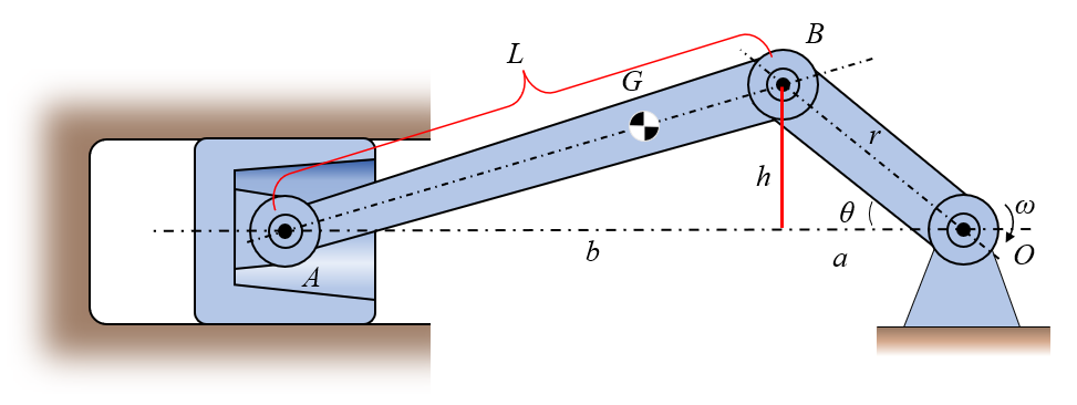
r = 50.0   # Crank length
L = 150.0  # Connecting rod length

def constraint_equations(vars, theta):
    """Constraint equations for crank-slider mechanism."""
    phi, x_A = vars
    rr_OB = r * np.array([-np.cos(theta), np.sin(theta)])
    rr_BA = L * np.array([np.cos(phi), np.sin(phi)])
    rr_OA_computed = rr_OB + rr_BA
    rr_OA_constraint = np.array([x_A, 0])
    return rr_OA_computed - rr_OA_constraint

# Prepare animation data
theta_range = np.linspace(0, 2*np.pi, 60)
solutions = []
initial_guess = [np.deg2rad(180), -150]

for theta in theta_range:
    sol = scipy.optimize.fsolve(constraint_equations, initial_guess, args=(theta,))
    solutions.append((theta, sol[0], sol[1]))  # (theta, phi, x_A)
    initial_guess = sol

fig, ax = plt.subplots(figsize=(12, 6))

def plot_mechanism(theta, phi, x_A):
    """Plot the crank-slider mechanism for given configuration."""
    ax.clear()
    
    # Calculate positions
    O = np.array([0, 0])
    B = r * np.array([-np.cos(theta), np.sin(theta)])
    A = np.array([x_A, 0])
    
    # Plot ground
    ground_x = np.linspace(-250, 50, 100)
    ax.plot(ground_x, np.zeros_like(ground_x), 'k-', linewidth=3, alpha=0.3)
    
    # Plot slider rail
    ax.plot([-250, 50], [0, 0], 'k-', linewidth=5)
    
    # Plot crank OB
    ax.plot([O[0], B[0]], [O[1], B[1]], 'b-o', linewidth=3, markersize=8, label='Crank')
    
    # Plot connecting rod BA
    ax.plot([B[0], A[0]], [B[1], A[1]], 'r-o', linewidth=3, markersize=8, label='Connecting rod')
    
    # Plot slider
    slider_width = 20
    slider_height = 15
    slider_rect = plt.Rectangle((x_A - slider_width/2, -slider_height/2), 
                                slider_width, slider_height, 
                                facecolor='green', edgecolor='black', linewidth=2)
    ax.add_patch(slider_rect)
    
    # Plot origin
    ax.plot(O[0], O[1], 'ko', markersize=10, label='O (origin)')
    
    # Labels
    ax.text(B[0] + 5, B[1] + 5, 'B', fontsize=12, fontweight='bold')
    ax.text(A[0], A[1] + 10, 'A', fontsize=12, fontweight='bold')
    ax.text(O[0] - 10, O[1] + 10, 'O', fontsize=12, fontweight='bold')
    
    # Settings
    ax.set_xlim(-220, 60)
    ax.set_ylim(-80, 80)
    ax.set_aspect('equal', adjustable='box')
    ax.grid(True, alpha=0.3)
    ax.set_xlabel('x [mm]')
    ax.set_ylabel('y [mm]')
    ax.set_title(f'Crank-Slider Mechanism (θ = {np.rad2deg(theta):.1f}°, φ = {np.rad2deg(phi):.1f}°)')
    ax.legend(loc='upper right')

def animate(frame_idx):
    """Animation function."""
    theta, phi, x_A = solutions[frame_idx]
    plot_mechanism(theta, phi, x_A)

# Create animation
plt.close(fig)
anim = FuncAnimation(fig, animate, frames=len(solutions), 
                     interval=50, repeat=True)

# Convert to HTML5 video
video_html = anim.to_html5_video()
video_html = video_html.replace('controls', 'controls autoplay loop muted')
video_html = video_html.replace('<video ', '<video style="width: 100%; height: auto;" ')
HTML(video_html)