Code
import numpy as np
import matplotlib.pyplot as plt
import mechanicskit as mkpatch() ExamplesThis notebook demonstrates the patch() function for visualizing finite element meshes, truss structures, and field data.
import numpy as np
import matplotlib.pyplot as plt
import mechanicskit as mk# Node coordinates (mm)
P = np.array([[0, 0],
[500, 0],
[300, 300],
[600, 300]])
# Element connectivity (1-based node numbers)
edges = np.array([[1, 2],
[1, 3],
[2, 3],
[2, 4],
[3, 4]])
U = np.array([[ 0. , 0. ],
[-0.1984, 0. ],
[ 0.2466, 0.09 ],
[ 0.445 , -0.9116]])
U_res = np.sqrt(U[:, 0]**2 + U[:, 1]**2)fig, ax = plt.subplots(figsize=(8, 6))
mk.patch('Faces', edges, 'Vertices', P, 'LineWidth', 2)
ax.plot(P[:, 0], P[:, 1], 'o', color='cyan',
markeredgecolor='black', markersize=14)
ax.axis('equal')
ax.axis('off')
ax.set_title('Basic Truss')
plt.show()
Visualize element forces with flat coloring (one color per element).
# Element forces (N)
forces = np.array([6052.76, -5582.25, -7274.51, 6380.16, -9912.07])

fig, ax = plt.subplots(figsize=(8, 6))
mk.patch('Faces', edges, 'Vertices', P,
      'FaceVertexCData', forces,
      'FaceColor', 'flat',
      'LineWidth', 3,
      'cmap', 'RdBu_r')  # Red for tension, blue for compression

mk.cmap('RdBu_r', label="Element forces", shrink=0.8)

ax.axis('equal')
ax.axis('off')
ax.set_title('Element Forces (Flat Colors)')
plt.show()

print(f"Force range: {forces.min():.1f} to {forces.max():.1f} N")
Force range: -9912.1 to 6380.2 NVisualize nodal temperatures with interpolated coloring.
scale = 50
P_deformed = P + scale * U

fig, ax = plt.subplots(figsize=(8, 6))

mk.patch('Faces', edges, 'Vertices', P)

mk.patch('Faces', edges, 'Vertices', P_deformed,
      'FaceVertexCData', U_res,
      'FaceColor', 'interp',
      'LineWidth', 4,
      'cmap', 'jet')

mk.cmap('jet', label="Displacement Magnitude (mm)", shrink=0.8)


ax.axis('equal')
ax.axis('off')
ax.set_title('Nodal Temperatures (Interpolated Colors)')
plt.show()
fig, ax = plt.subplots(figsize=(8, 6))
mk.patch('Faces', edges, 'Vertices', P,
      'FaceVertexCData', forces,
      'FaceColor', 'flat',
      'LineWidth', 4,
      'FaceAlpha', 0.5)
ax.plot(P[:, 0], P[:, 1], 'o', color='red',
        markeredgecolor='black', markersize=14)
ax.axis('equal')
ax.axis('off')
ax.set_title('Semi-Transparent Elements (alpha=0.5)')
plt.show()
# 3D node coordinates
P_3d = np.array([[0, 0, 0],
                 [500, 0, 0],
                 [300, 300, 0],
                 [600, 300, 0],
                 [300, 150, 400]])

# 3D element connectivity
edges_3d = np.array([[1, 2],
                     [1, 3],
                     [2, 3],
                     [2, 4],
                     [3, 4],
                     [1, 5],
                     [2, 5],
                     [3, 5],
                     [4, 5]])

# 3D element forces
forces_3d = np.array([100, -80, 50, -120, 90, -150, 110, -95, 130])

fig = plt.figure(figsize=(10, 8))
ax = fig.add_subplot(111, projection='3d')
mk.patch('Faces', edges_3d, 'Vertices', P_3d,
      'FaceVertexCData', forces_3d,
      'LineWidth', 2,
      'cmap', 'coolwarm',
      ax=ax)
ax.scatter(P_3d[:, 0], P_3d[:, 1], P_3d[:, 2],
          color='yellow', edgecolor='black', s=100)
ax.set_xlabel('X (mm)')
ax.set_ylabel('Y (mm)')
ax.set_zlabel('Z (mm)')
ax.set_title('3D Truss with Element Forces')
plt.show()
# Triangular mesh vertices
vertices_2d = np.array([[0, 0],
                        [1, 0],
                        [0.5, 0.866],
                        [1.5, 0.866],
                        [1, 1.732]])

# Triangle connectivity
faces_2d = np.array([[1, 2, 3],
                     [2, 4, 3],
                     [3, 4, 5]])

# Per-element colors
face_colors = np.array([0.2, 0.5, 0.8])

fig, ax = plt.subplots(figsize=(8, 6))
mk.patch('Faces', faces_2d, 'Vertices', vertices_2d,
      'FaceVertexCData', face_colors,
      'FaceColor', 'flat',
      'EdgeColor', 'black',
      'LineWidth', 2,
      'cmap', 'plasma')
ax.plot(vertices_2d[:, 0], vertices_2d[:, 1], 'ko', markersize=8)
ax.set_aspect('equal')
ax.set_title('2D Triangular Elements')
plt.colorbar(ax.collections[0], ax=ax, label='Element Value')
plt.show()
# 3D quad vertices
vertices_3d_surf = np.array([[0, 0, 0],
                             [1, 0, 0],
                             [1, 1, 0],
                             [0, 1, 0]])

# Quad face
faces_3d_surf = np.array([[1, 2, 3, 4]])

fig = plt.figure(figsize=(8, 6))
ax = fig.add_subplot(111, projection='3d')
mk.patch('Faces', faces_3d_surf, 'Vertices', vertices_3d_surf,
      'FaceColor', 'red',
      'FaceAlpha', 0.6,
      'EdgeColor', 'black',
      'LineWidth', 2,
      ax=ax)
ax.scatter(vertices_3d_surf[:, 0], vertices_3d_surf[:, 1], vertices_3d_surf[:, 2],
          color='blue', s=100)
ax.set_xlabel('X')
ax.set_ylabel('Y')
ax.set_zlabel('Z')
ax.set_title('3D Quad Surface (Transparent)')
plt.show()
# More complex mesh for advanced examples
P_quad = np.array([[0, 0],
                   [3, 0],
                   [3, 1.2],
                   [0, 1.2],
                   [0.7, 0],
                   [1.6, 0],
                   [2.5, 0],
                   [3, 0.5],
                   [2.3, 1.2],
                   [1.5, 1.2],
                   [0.6, 1.2],
                   [0, 0.5],
                   [0.55, 0.4],
                   [1.45, 0.6],
                   [2.4, 0.45]])

nodes_quad = np.array([[1, 5, 13, 12],
                       [12, 13, 11, 4],
                       [5, 6, 14, 13],
                       [13, 14, 10, 11],
                       [14, 15, 9, 10],
                       [6, 7, 15, 14],
                       [7, 2, 8, 15],
[15, 8, 3, 9]])fig, ax = plt.subplots(figsize=(10, 6))
# Draw mesh with cyan faces
mk.patch('Faces', nodes_quad, 'Vertices', P_quad,
'FaceColor', 'cyan',
'EdgeColor', 'black',
'EdgeAlpha', 0.3,
'LineWidth', 1.5,
ax=ax)
# Plot nodes
ax.plot(P_quad[:, 0], P_quad[:, 1], 'ok', markerfacecolor='black', markersize=16)
# Label nodes
for i in range(len(P_quad)):
ax.text(P_quad[i, 0], P_quad[i, 1], str(i+1),
color='w', fontsize=8, ha='center', va='center')
# Label elements at their centroids
for iel in range(len(nodes_quad)):
element_nodes = nodes_quad[iel] - 1 # Convert to 0-based
xm = np.mean(P_quad[element_nodes, 0])
ym = np.mean(P_quad[element_nodes, 1])
ax.text(xm, ym, str(iel+1), fontsize=9, ha='center', va='center')
ax.axis('equal')
ax.set_title('Quad Element Mesh with Labels')
plt.show()
# Create synthetic displacement field (simulating FEM results)
np.random.seed(42)
u_flat = np.zeros(2 * len(P_quad))

# Simulate bending: displacement increases with x, varies with y
for i in range(len(P_quad)):
    x, y = P_quad[i]
    u_flat[2*i] = 0.15 * x * (1 + 0.3 * y)      # x-displacement
    u_flat[2*i+1] = -0.05 * x**2 / 9            # y-displacement

# Convert to nodal displacement array (n_nodes, 2)
U = np.column_stack([u_flat[0::2], u_flat[1::2]])

# Compute displacement magnitude at each node
UR = np.sqrt(np.sum(U**2, axis=1))

# Scale factor for visualization
scale = 1.0

fig, ax = plt.subplots(figsize=(10, 6))

# Draw deformed mesh with displacement magnitude colors
mk.patch('Faces', nodes_quad, 'Vertices', P_quad + U * scale,
      'FaceVertexCData', UR,
      'FaceColor', 'interp',
      'EdgeColor', 'black',
      'EdgeAlpha', 0.5,
      'LineWidth', 1.0,
      'cmap', 'jet',
      ax=ax)

ax.axis('equal')
ax.set_title(f'Displacement Field, scale: {scale}')
plt.colorbar(ax.collections[0], ax=ax, label='Displacement Magnitude')
plt.show()

print(f"Displacement range: {UR.min():.4f} to {UR.max():.4f}")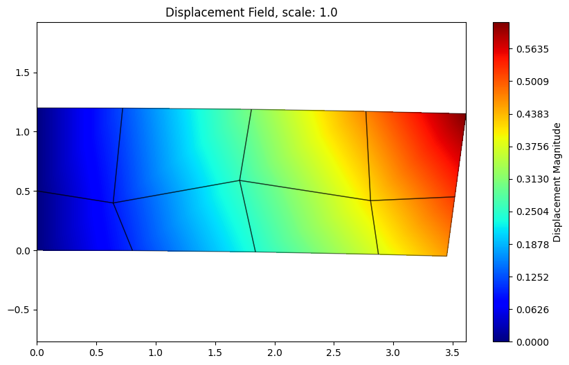
Displacement range: 0.0000 to 0.6140# Create synthetic stress data (one value per element)
element_stresses = np.array([150, -80, 200, -120, 180, 90, -150, 110])
fig, ax = plt.subplots(figsize=(10, 6))
# Draw mesh with per-element colors
mk.patch('Faces', nodes_quad, 'Vertices', P_quad,
'FaceVertexCData', element_stresses,
'FaceColor', 'flat',
'EdgeColor', 'black',
'LineWidth', 2,
'cmap', 'RdBu_r', # Red for tension, blue for compression
ax=ax)
# Plot nodes
ax.plot(P_quad[:, 0], P_quad[:, 1], 'ok', markerfacecolor='yellow',
markeredgecolor='black', markersize=10)
ax.axis('equal')
ax.set_title('Element Stress Field (Flat Colors)')
plt.colorbar(ax.collections[0], ax=ax, label='Stress (MPa)')
plt.show()
print(f"Stress range: {element_stresses.min():.1f} to {element_stresses.max():.1f} MPa")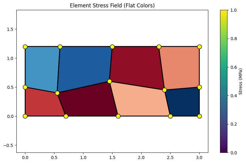
Stress range: -150.0 to 200.0 MPa# Create synthetic temperature data (one value per node)
node_temps_quad = np.zeros(len(P_quad))
for i in range(len(P_quad)):
x, y = P_quad[i]
# Temperature increases from left to right
node_temps_quad[i] = 100 * (x / 3.0) + 20
fig, ax = plt.subplots(figsize=(10, 6))
# Draw mesh with interpolated nodal temperatures
mk.patch('Faces', nodes_quad, 'Vertices', P_quad,
'FaceVertexCData', node_temps_quad,
'FaceColor', 'interp',
'EdgeColor', 'black',
'LineWidth', 1.5,
'cmap', 'hot',
ax=ax)
# Plot nodes
# ax.plot(P_quad[:, 0], P_quad[:, 1], 'ok', markerfacecolor='cyan',
# markeredgecolor='black', markersize=10)
ax.axis('equal')
ax.set_title('Temperature Field (Interpolated Colors)')
plt.colorbar(ax.collections[0], ax=ax, label='Temperature (°C)')
plt.show()
print(f"Temperature range: {node_temps_quad.min():.1f} to {node_temps_quad.max():.1f} °C")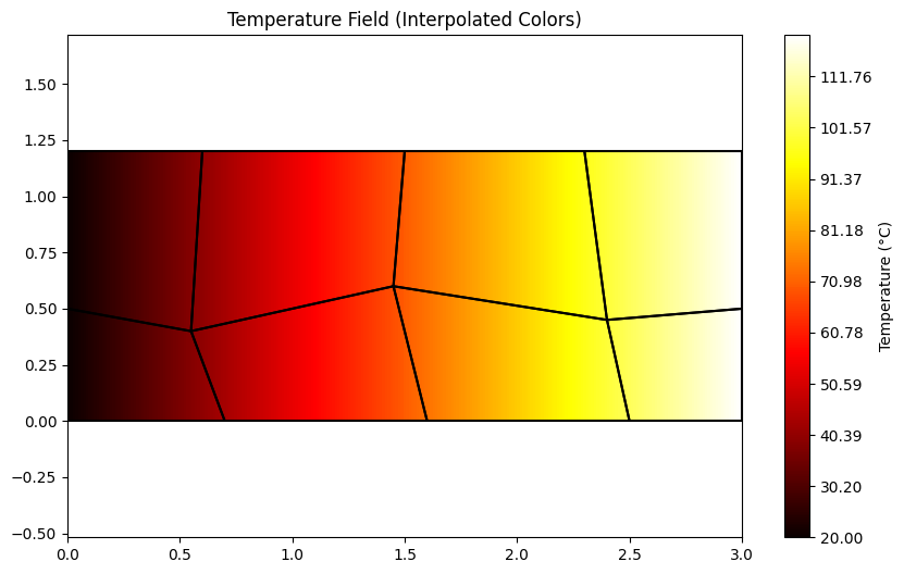
Temperature range: 20.0 to 120.0 °Cfig, axes = plt.subplots(1, 3, figsize=(16, 5))
collections = []
for idx, scale in enumerate([0.5, 1.0, 2.0]):
ax = axes[idx]
# Original mesh (light gray)
mk.patch('Faces', nodes_quad, 'Vertices', P_quad,
'FaceColor', 'white',
'EdgeColor', 'gray',
'EdgeAlpha', 0.3,
'LineWidth', 1.0,
ax=ax)
# Deformed mesh
P_def = P_quad + U * scale
pc = mk.patch('Faces', nodes_quad, 'Vertices', P_def,
'FaceVertexCData', UR,
'FaceColor', 'interp',
'EdgeColor', 'black',
'EdgeAlpha', 0.2,
'LineWidth', 1.5,
'cmap', 'viridis',
ax=ax)
collections.append(pc)
ax.axis('equal')
ax.set_title(f'Scale: {scale}')
# Add shared colorbar
# fig.colorbar(collections[0], ax=axes.ravel().tolist(), label='Displacement Magnitude', pad=0.02)
mk.cmap('viridis', label="Displacement Magnitude", shrink=0.8)
plt.suptitle('Displacement Field at Different Scales', fontsize=14)
plt.tight_layout()
plt.show()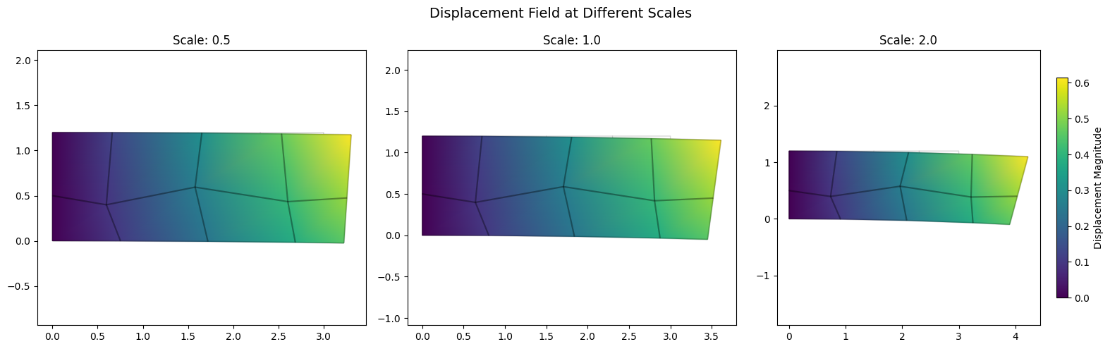
fig, axes = plt.subplots(1, 3, figsize=(15, 5))

for idx, alpha in enumerate([0.3, 0.6, 1.0]):
    ax = axes[idx]

    mk.patch('Faces', nodes_quad, 'Vertices', P_quad,
          'FaceVertexCData', element_stresses,
          'FaceColor', 'flat',
          'FaceAlpha', alpha,
          'EdgeColor', 'black',
          'LineWidth', 2,
          'cmap', 'plasma',
          ax=ax)

    # ax.plot(P_quad[:, 0], P_quad[:, 1], 'ok', markerfacecolor='white',
    #         markeredgecolor='black', markersize=8)

    ax.axis('equal')
    ax.set_title(f'FaceAlpha: {alpha}')

plt.suptitle('Face Transparency Variations', fontsize=14)
plt.tight_layout()
plt.show()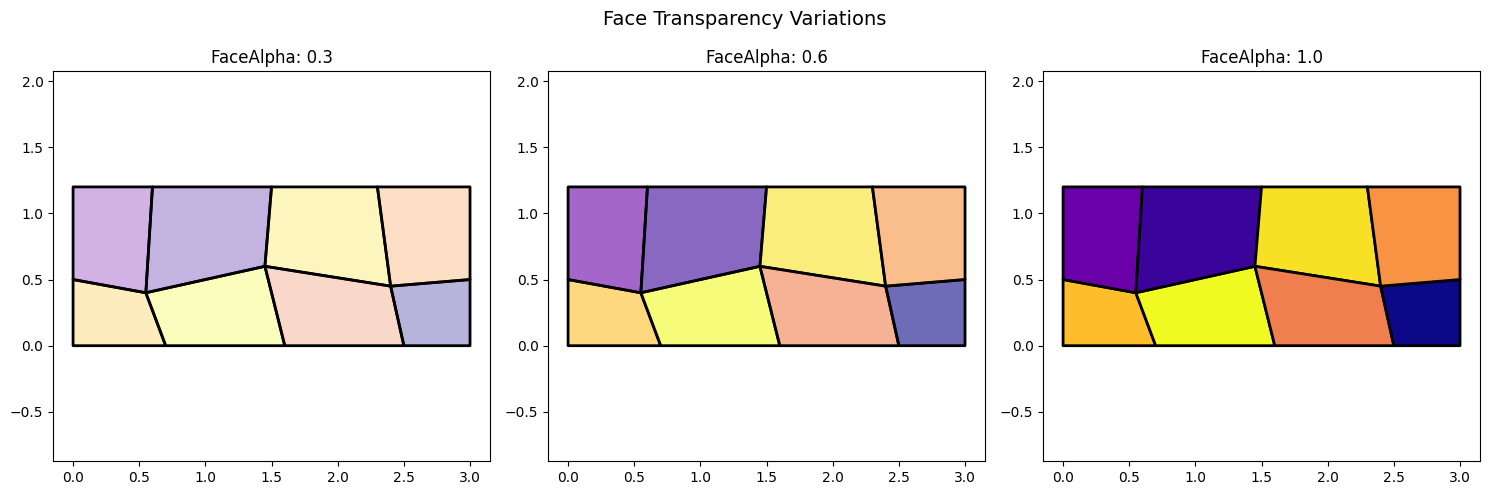
The patch() function provides flexible visualization for FEM:
'flat', 'interp', or explicit color)'viridis', 'hot', 'RdBu_r')'flat': One color per element (use with per-element data)'interp': Interpolated colors (use with per-node data)FaceColor='flat' with per-element dataFaceColor='interp' with per-node dataP + U * scale