What if your report could move? What if your reader could drag a slider and watch your simulation respond in real-time? What if your convergence plot let them zoom in on the interesting region?
This is the power of HTML reports.
While PDFs are the gold standard for formal submissions, HTML reports unlock a dimension that static documents simply cannot reach: interactivity. Your animations play automatically. Your plots respond to mouse hovers. Your readers can explore your data instead of just viewing it.
And the best part? You write the same notebook, just render to HTML instead of PDF.
When to Use HTML vs PDF
Consideration
Choose PDF
Choose HTML
Formal submission
Required for journals, theses
Usually not accepted
Animations
Static frames only
Full motion, autoplay
Interactive plots
Not possible
Zoom, pan, hover tooltips
Sharing online
Requires download
Opens in any browser
File size
Compact
Can be large with media
Printing
Designed for print
May not print well
Canvas/LMS upload
Standard
Also works
LaTeX installation
Required
Not needed
Rule of thumb:
Use PDF for formal academic submissions
Use HTML when your work includes animations, simulations, or interactive visualizations, or when you want to share online
Tip
You can upload HTML files to Canvas just like PDFs! This gives your instructor a richer view of your work. Some even prefer it for computational assignments.
Embedding Animations
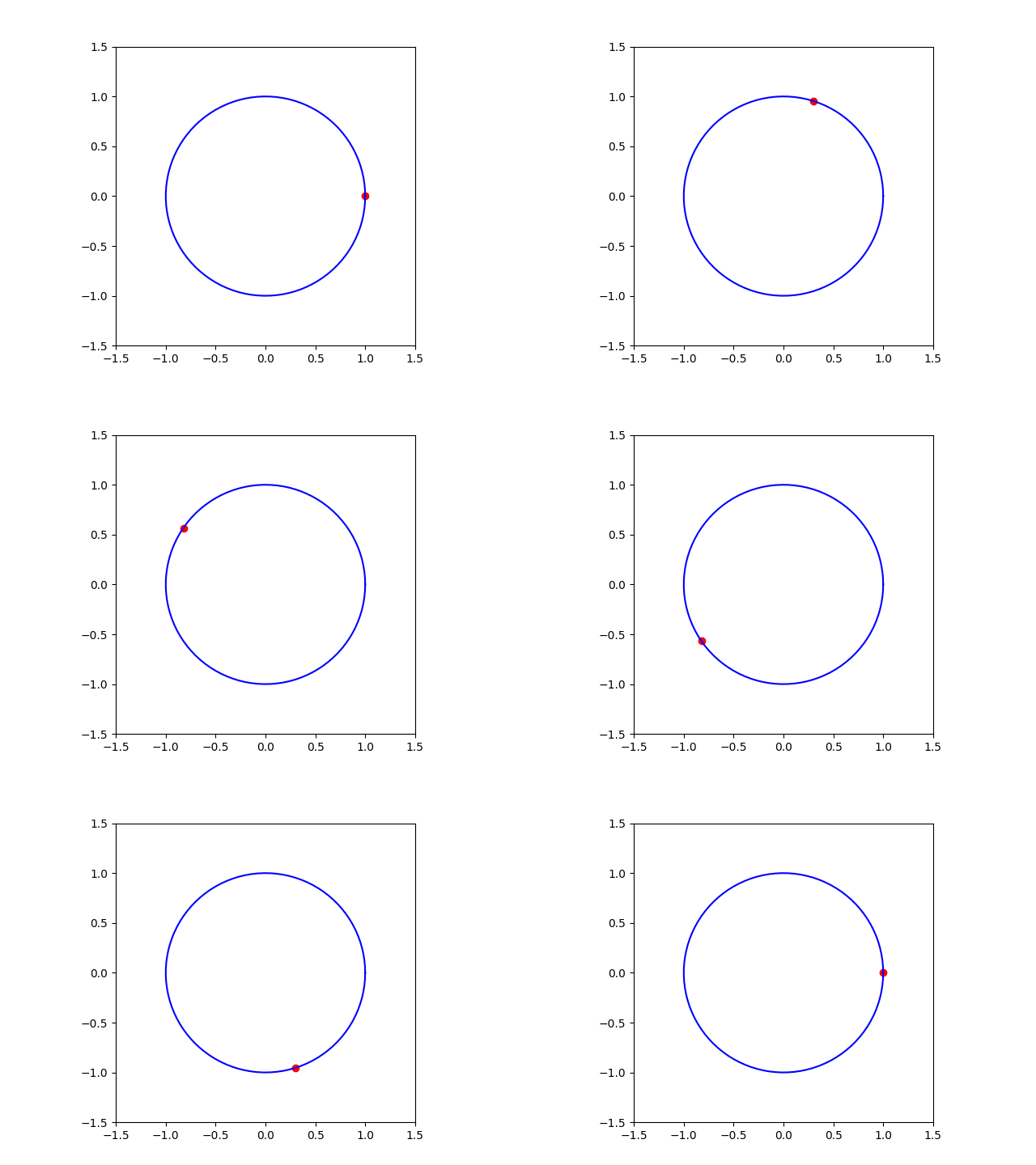
Let’s make a report come alive. We’ll animate a point moving around a circle using three different approaches, each with its own trade-offs.
Approach 1: GIF for Quick and Simple Animations
GIFs are the easiest way to add animation. They work everywhere and require minimal code. The downside? They’re inefficient (large files) and have limited color depth (256 colors).
Best for: Quick demos, simple animations, maximum compatibility.
The circle is given by the parametric equations:
\[
x(t) = r\cos(t), \quad y(t) = r\sin(t)
\]
where \(t \in [0, 2\pi]\) and \(r = 1\).
Code
import numpy as npimport matplotlib.pyplot as pltimport matplotlib.animation as animationfig, ax = plt.subplots()line, = ax.plot([], [], 'ro')ax.set_xlim(-1.5, 1.5)ax.set_ylim(-1.5, 1.5)t = np.linspace(0, 2*np.pi, 100)y = np.sin(t)x = np.cos(t)ax.plot(x, y, 'b-')ax.set_aspect('equal', 'box')def update(frame): x = np.cos(frame) y = np.sin(frame) line.set_data([x], [y])return line,ani = animation.FuncAnimation(fig, update, frames=t, blit=True)plt.close()ani.save('circle_animation.gif', writer='pillow')
Embed the GIF using standard markdown:

Circle Animation
Warning
GIF files can be surprisingly large. A 5-second animation can easily exceed 1 MB. For longer or higher-quality animations, use MP4 instead.
Approach 2: MP4 Video for Better Quality
MP4 is superior to GIF in almost every respect: smaller files, better quality, full color, and playback controls. The only downside is you need ffmpeg installed.
Best for: Any animation longer than a few seconds, high-quality visuals, smooth playback.
Code
import numpy as npimport matplotlib.pyplot as pltimport matplotlib.animation as animationfig, ax = plt.subplots()line, = ax.plot([], [], 'ro')ax.set_xlim(-1.5, 1.5)ax.set_ylim(-1.5, 1.5)t = np.linspace(0, 2*np.pi, 360*2)y = np.sin(t)x = np.cos(t)ax.plot(x, y, 'b-')ax.set_aspect('equal', 'box')def update(frame): x = np.cos(frame) y = np.sin(frame) line.set_data([x], [y])return line,ani = animation.FuncAnimation(fig, update, frames=t, blit=True) plt.close()ani.save('circle_animation.mp4', writer='ffmpeg', fps=30, dpi=200)
Embed MP4 using HTML5 video tags with autoplay and loop:
This is where HTML truly shines. Instead of a passive video, you get an interactive player with a slider that lets you scrub through the animation frame by frame. Your reader can pause, rewind, and explore at their own pace.
Best for: Educational content, when readers need to study specific frames, exploratory analysis.
Code
import numpy as npimport matplotlib.pyplot as pltimport matplotlib.animation as animationfrom IPython.display import HTMLfig, ax = plt.subplots()line, = ax.plot([], [], 'ro')ax.set_xlim(-1.5, 1.5)ax.set_ylim(-1.5, 1.5)t = np.linspace(0, 2*np.pi, 60)y = np.sin(t)x = np.cos(t)ax.plot(x, y, 'b-')ax.set_aspect('equal', 'box')def update(frame): x = np.cos(frame) y = np.sin(frame) line.set_data([x], [y])return line,ani = animation.FuncAnimation(fig, update, frames=t, blit=True)plt.close()html_content = ani.to_jshtml(default_mode='loop')HTML(f"""<div style="width:100%"><style>img {{ max-width: 100% !important; }}</style>{html_content}</div><script>setTimeout(() => document.querySelector('button[title="Play"]')?.click(), 100);</script>""")
Warning
JS-HTML animations embed each frame as a base64 image, so file size grows quickly. Keep frame counts reasonable (< 100 frames). For longer animations, use MP4.
You can simplify the boilerplate using MechanicsKit:
import mechanicskit as mkmk.to_responsive_html(ani, container_id='my-animation')
Interactive Plots with Plotly
Static matplotlib plots are fine, but what if your reader could zoom in on that interesting spike, or hover over a point to see its exact value? Plotly makes this trivial.
Code
import plotly.express as pximport plotly.io as pioimport numpy as npimport pandas as pd# Required for VSCode + Quarto compatibilitypio.renderers.default ="plotly_mimetype+notebook_connected"# Generate some datanp.random.seed(42)n =100df = pd.DataFrame({'x': np.linspace(0, 10, n),'y': np.sin(np.linspace(0, 10, n)) +0.1*np.random.randn(n),'category': np.random.choice(['A', 'B', 'C'], n)})fig = px.scatter(df, x='x', y='y', color='category', title='Interactive Scatter Plot: Try zooming and hovering!', hover_data=['x', 'y'])fig.show()
Try it: click and drag to zoom, double-click to reset, hover over points to see values.
Plotly works seamlessly with Quarto HTML output. Install with:
uv pip install plotly
Rendering to HTML
To create a self-contained HTML file with all media embedded:
quarto render my_report.ipynb --to html --embed-resources
GitHub Pages is perfect for project documentation, course materials, or sharing computational notebooks with colleagues who don’t have Python installed.