3.9 PDF Reports with LaTeX
Writing clear, professional reports is an essential skill for engineers and scientists. Your findings are only as valuable as your ability to communicate them. This guide teaches you to create publication-quality PDF reports with properly typeset mathematics, automatically numbered figures and equations, and integrated code, all without the complexity of traditional LaTeX.
Why Quarto + LaTeX?
Most LaTeX tutorials and resources assume you’re writing a standalone .tex document. This requires extensive boilerplate code just to get started:
\documentclass{article}
\usepackage{amsmath}
\usepackage{graphicx}
\usepackage{hyperref}
\begin{document}
\title{My Report}
\author{Name}
\maketitle
% Finally, your content here...
\end{document}
With Quarto, you write in simple markdown, use LaTeX only for mathematics, and get all the power of a full LaTeX document with none of the ceremony. Better still, you can include executable Python code that generates your figures and tables automatically.
| Approach | Math Support | Code Integration | Version Control | Setup Complexity |
|---|---|---|---|---|
| Word/Google Docs | Poor | None | Difficult | Easy |
| Overleaf | Excellent | None | Limited | Medium |
| Pure LaTeX | Excellent | Manual | Good | High |
| Quarto + LaTeX | Excellent | Native | Excellent | Low |
Prerequisites
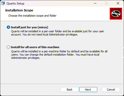
Install Quarto
Download from the Quarto website. If you don’t have admin rights (e.g., on a university computer), select “Install for me only”.
LaTeX Distribution (for PDF output)
To generate PDFs, you need a LaTeX distribution. Quarto will use any of these:
TeX Live (Linux): Often pre-installed. Install with
sudo apt install texlive-fullMacTeX (macOS): Full distribution from tug.org/mactex
MiKTeX (Windows): From miktex.org
TinyTeX: Lightweight option (~250 MB) that Quarto can install:
quarto install tinytex
Check if you already have LaTeX: pdflatex --version
If you’re on a university computer, LaTeX is likely already installed. TinyTeX is mainly useful for personal machines where you want a minimal install.
Install VS Code + Extensions
- Install VS Code
- Install the Quarto extension from the Extensions marketplace
- Install the Jupyter extension for notebook support
Follow the Python installation guide to set up Python and Jupyter.
LaTeX Mathematics Essentials
LaTeX is the standard for typesetting mathematics in scientific documents. In Quarto, you use LaTeX syntax only for math: no document preamble, no \begin{document}, just the equations themselves.
Inline vs Display Math
Use single dollar signs $...$ for inline math and double dollar signs $$...$$ for display (centered) equations:
| Syntax | Result | Use for |
|---|---|---|
$x^2 + y^2 = r^2$ |
\(x^2 + y^2 = r^2\) | Math within text |
$$x^2 + y^2 = r^2$$ |
(centered equation) | Standalone equations |
\[x^2 + y^2 = r^2\]
Common Mathematical Notation
Fractions and Roots
| LaTeX | Result | Description |
|---|---|---|
\frac{a}{b} |
\(\frac{a}{b}\) | Fraction |
\dfrac{a}{b} |
\(\dfrac{a}{b}\) | Display-style fraction |
\sqrt{x} |
\(\sqrt{x}\) | Square root |
\sqrt[n]{x} |
\(\sqrt[n]{x}\) | nth root |
Subscripts, Superscripts, and Accents
| LaTeX | Result | Description |
|---|---|---|
x^2 |
\(x^2\) | Superscript |
x_i |
\(x_i\) | Subscript |
x_i^2 |
\(x_i^2\) | Both |
x_{i,j} |
\(x_{i,j}\) | Multi-character subscript |
\hat{x} |
\(\hat{x}\) | Hat accent |
\bar{x} |
\(\bar{x}\) | Bar accent |
\dot{x} |
\(\dot{x}\) | Dot (time derivative) |
\ddot{x} |
\(\ddot{x}\) | Double dot |
\vec{v} |
\(\vec{v}\) | Vector arrow |
\mathbf{A} |
\(\mathbf{A}\) | Bold (for vectors/matrices) |
\boldsymbol{\sigma} |
\(\boldsymbol{\sigma}\) | Bold (for tensors/ greek letters) |
Greek Letters
| LaTeX | Result | LaTeX | Result |
|---|---|---|---|
\alpha |
\(\alpha\) | \beta |
\(\beta\) |
\gamma |
\(\gamma\) | \delta |
\(\delta\) |
\epsilon |
\(\epsilon\) | \theta |
\(\theta\) |
\lambda |
\(\lambda\) | \mu |
\(\mu\) |
\pi |
\(\pi\) | \sigma |
\(\sigma\) |
\phi |
\(\phi\) | \omega |
\(\omega\) |
\Gamma |
\(\Gamma\) | \Delta |
\(\Delta\) |
\Omega |
\(\Omega\) | \Sigma |
\(\Sigma\) |
Operators and Relations
| LaTeX | Result | LaTeX | Result |
|---|---|---|---|
\times |
\(\times\) | \cdot |
\(\cdot\) |
\pm |
\(\pm\) | \mp |
\(\mp\) |
\leq |
\(\leq\) | \geq |
\(\geq\) |
\neq |
\(\neq\) | \approx |
\(\approx\) |
\equiv |
\(\equiv\) | \propto |
\(\propto\) |
\rightarrow |
\(\rightarrow\) | \Rightarrow |
\(\Rightarrow\) |
\partial |
\(\partial\) | \nabla |
\(\nabla\) |
\infty |
\(\infty\) | \forall |
\(\forall\) |
Sums, Products, and Integrals
These “big operators” take limits that appear differently in inline vs display mode:
$$\sum_{i=1}^{n} x_i \qquad \prod_{i=1}^{n} x_i \qquad \int_{a}^{b} f(x)\,dx$$\[\sum_{i=1}^{n} x_i \qquad \prod_{i=1}^{n} x_i \qquad \int_{a}^{b} f(x)\,dx\]
| LaTeX | Result | Description |
|---|---|---|
\sum_{i=1}^{n} |
\(\sum_{i=1}^{n}\) | Summation |
\prod_{i=1}^{n} |
\(\prod_{i=1}^{n}\) | Product |
\int_{a}^{b} |
\(\int_{a}^{b}\) | Integral |
\oint |
\(\oint\) | Contour integral |
\iint |
\(\iint\) | Double integral |
\lim_{x \to 0} |
\(\lim_{x \to 0}\) | Limit |
Use \, to add a thin space before dx in integrals: \int f(x)\,dx looks better than \int f(x)dx.
Matrices and Vectors
Matrices use the pmatrix (parentheses), bmatrix (brackets), or vmatrix (vertical bars for determinants) environments:
$$\mathbf{A} = \begin{pmatrix} a & b \\ c & d \end{pmatrix}, \quad
\mathbf{x} = \begin{bmatrix} x_1 \\ x_2 \\ x_3 \end{bmatrix}, \quad
\det(\mathbf{A}) = \begin{vmatrix} a & b \\ c & d \end{vmatrix}$$
\[\mathbf{A} = \begin{pmatrix} a & b \\ c & d \end{pmatrix}, \quad \mathbf{x} = \begin{bmatrix} x_1 \\ x_2 \\ x_3 \end{bmatrix}, \quad \det(\mathbf{A}) = \begin{vmatrix} a & b \\ c & d \end{vmatrix}\]
- Use
&to separate columns - Use
\\to start a new row
Multi-line Equations with Alignment
Use the align environment to align multiple equations at the & symbol:
$$\begin{align}
f(x) &= (x+1)^2 \\
     &= x^2 + 2x + 1
\end{align}$$
\[\begin{align} f(x) &= (x+1)^2 \\ &= x^2 + 2x + 1 \end{align}\]
Cases might be useful for system of ODEs or piecewise functions:
$$\begin{cases}
\frac{dy}{dt}=y_{2}\\[6pt]
\frac{dy_{2}}{dt}=-cy_{2}-ky
\end{cases}$$
\[\begin{cases} \frac{dy}{dt}=y_{2}\\[6pt] \frac{dy_{2}}{dt}=-cy_{2}-ky \end{cases}\]
Notice the extra space added with [6pt] for readability.
Equation Labels and Cross-References
Add {#eq-label} after an equation to create a reference:
The fundamental theorem states:
$$F(b) - F(a) = \int_a^b f(x)\,dx$$ {#eq-ftc}

As shown in @eq-ftc, the integral equals...
Quarto automatically numbers equations and creates clickable links.
Your First Report
The Workflow
- Create a Jupyter Notebook (
.ipynb) in VS Code - Add a cell at the top with YAML front matter
- Write markdown text with LaTeX equations
- Add Python code cells for figures and calculations
- Render to PDF with:
quarto render my_report.ipynb --to pdf
YAML Front Matter
The first cell of your notebook should contain YAML front matter with the document configuration. We really do not need any of this front matter for quarto to render a PDF. This works in either a raw cell or a markdown cell:
---
title: "Your Report Title"
subtitle: "Optional Subtitle"
author: "Your Name"
date: today
lang: en
format:
  pdf:
    documentclass: article
    papersize: a4
    geometry: margin=2.5cm
    fontsize: 11pt
    number-sections: true
    colorlinks: true
jupyter: python3
---
Key options:
| Option | Description |
|---|---|
title |
Document title |
subtitle |
Subtitle displayed below the title |
author |
Author name(s) |
date |
Date (use today for current date) |
description |
Brief description (appears in PDF metadata) |
lang |
Document language (e.g., sv for Swedish, en for English) |
documentclass |
article (short), report (longer with chapters), book |
papersize |
Paper size: a4, letter, a5, etc. |
geometry |
Page margins (e.g., margin=2.5cm or margin=1in) |
fontsize |
Base font size: 10pt, 11pt, or 12pt |
number-sections |
Automatically number headings |
number-equations |
Automatically number display equations |
colorlinks |
Make hyperlinks colored instead of boxed |
toc |
Add table of contents |
include-in-header |
Add LaTeX packages (see below) |
Adding LaTeX Packages
Need \bm for bold math symbols or other LaTeX packages? Use include-in-header:
---
title: "My Report"
format:
  pdf:
    include-in-header:
      text: |
        \usepackage{bm}
        \usepackage{siunitx}
---
Now you can use $\bm{\sigma}$ for bold tensors: \(\boldsymbol{\sigma}\)
Common packages to add:
| Package | Provides |
|---|---|
bm |
\bm{} for bold math (better than \boldsymbol) |
siunitx |
\SI{9.8}{m/s^2} for units |
cancel |
\cancel{x} for crossed-out terms |
physics |
\dv{f}{x}, \pdv{f}{x} for derivatives |
Not all LaTeX packages are compatible with Quarto’s HTML rendering. For instance, Quarto uses MathJax or KaTeX for rendering math in HTML, wich does not support for bold symbols.
Including Code and Figures
One of Quarto’s greatest strengths is seamless code integration. Your Python code runs during rendering, and its output (plots, tables) is automatically included in the PDF.
Controlling Code Display
Use special comments (#|) at the top of code cells:
#| label: fig-example
#| fig-cap: "A sine wave with period 2π"
#| echo: false

import numpy as np
import matplotlib.pyplot as plt

x = np.linspace(0, 2*np.pi, 100)
plt.plot(x, np.sin(x))
plt.xlabel('x')
plt.ylabel('sin(x)')
plt.show()| Option | Effect |
|---|---|
#| echo: false |
Hide code, show only output |
#| echo: true |
Show code (default) |
#| output: false |
Hide output |
#| label: fig-name |
Create referenceable figure |
#| fig-cap: "..." |
Figure caption |
#| warning: false |
Suppress warnings |
Referencing Figures
After labeling a figure, reference it in your text:
As shown in @fig-example, the sine function oscillates between -1 and 1.Quarto handles numbering automatically. No need to manually track “Figure 1”, “Figure 2”, etc.
Citations and References
You can define references directly in the YAML front matter:
---
title: "My Report"
references:
  - id: newton1687
    type: book
    author:
      - family: Newton
        given: Isaac
    title: Philosophiæ Naturalis Principia Mathematica
    issued:
      year: 1687
---
Then cite in your text using @id:
Newton's laws of motion @newton1687 form the foundation of classical mechanics.This renders as: “Newton’s laws of motion (Newton, 1687) form the foundation…” with the full reference automatically added at the end.
For documents with many references, use an external .bib file instead. See the Quarto citation documentation.
Complete Example
Let’s walk through a complete report for a numerical integration problem.
The Problem
Evaluate the integral:
\[\int_{0}^{2} \frac{1}{\sqrt{1 + \sin^2(x)}} dx\]
Requirements:
- Compare Trapezoidal rule vs Gaussian quadrature
- Determine points needed for error < \(10^{-10}\)
- Create convergence plots
- Write a professional report with citations
The Generated PDF
Here is the rendered PDF output from the example report:
The Source Notebook
The report is built from a Jupyter notebook with these cells:
Cell 1 (Raw): YAML front matter with inline bibliography
---
title: "Numerical Integration: Trapezoidal Rule vs Gaussian Quadrature"
author: "Student Name"
date: today
format:
  pdf:
    documentclass: article
    geometry: margin=2.5cm
    fontsize: 11pt
    number-sections: true
jupyter: python3
references:
  - id: golubWelsch
    type: article-journal
    author:
      - family: Golub
        given: Gene H.
      - family: Welsch
        given: John H.
    title: Calculation of Gauss Quadrature Rules
    container-title: Mathematics of Computation
    volume: 23
    page: 221-230
    issued:
      year: 1969
---
Cell 2 (Markdown): Introduction with labeled equation
## Introduction

We seek to evaluate the integral

$$
I = \int_{0}^{2} \frac{1}{\sqrt{1 + \sin^2(x)}} \, dx
$$ {#eq-integral}

This integral does not have an elementary closed-form solution.
It is an *elliptic integral*. Therefore, we must use numerical methods.
Cell 3 (Code): Setup code (hidden in output)
#| label: setup
#| echo: false
#| output: false

import numpy as np
import matplotlib.pyplot as plt
from scipy import integrate

def f(x):
    return 1 / np.sqrt(1 + np.sin(x)**2)

I_ref, _ = integrate.quad(f, 0, 2)
Cell 4 (Markdown): Method descriptions with equations and citations
## Numerical Methods

### Trapezoidal Rule

The composite trapezoidal rule approximates the integral as:

$$
I \approx \frac{h}{2}\left[f(a) + 2\sum_{i=1}^{n-1}f(x_i) + f(b)\right]
$$ {#eq-trapz}

where $h = (b-a)/n$ is the step size.

### Gaussian Quadrature

Gaussian quadrature uses optimally chosen nodes and weights @golubWelsch:

$$
I \approx \sum_{i=1}^{n} w_i f(x_i)
$$ {#eq-gauss}
Cell 5 (Code): Convergence plot with caption
#| label: fig-convergence
#| fig-cap: "Convergence comparison: error vs number of points."
#| echo: false

def trapezoidal(f, a, b, n):
    x = np.linspace(a, b, n + 1)
    h = (b - a) / n
    return h * (0.5*f(x[0]) + np.sum(f(x[1:-1])) + 0.5*f(x[-1]))

def gauss_legendre(f, a, b, n):
    nodes, weights = np.polynomial.legendre.leggauss(n)
    x = 0.5*(b-a)*nodes + 0.5*(b+a)
    return 0.5*(b-a)*np.sum(weights*f(x))

n_trap = np.logspace(1, 4, 30).astype(int)
n_gauss = np.arange(2, 25)

err_trap = [abs(trapezoidal(f, 0, 2, n) - I_ref) for n in n_trap]
err_gauss = [abs(gauss_legendre(f, 0, 2, n) - I_ref) for n in n_gauss]

plt.figure(figsize=(8, 5))
plt.loglog(n_trap, err_trap, 'b-o', label='Trapezoidal')
plt.loglog(n_gauss, err_gauss, 'r-s', label='Gauss-Legendre')
plt.axhline(1e-10, color='k', linestyle='--', label='Target')
plt.xlabel('Number of points')
plt.ylabel('Absolute error')
plt.legend()
plt.grid(True, alpha=0.3)
plt.show()
Cell 6 (Markdown): Conclusion with cross-references
## Conclusion

Gaussian quadrature dramatically outperforms the trapezoidal rule.
As shown in @fig-convergence, Gaussian quadrature achieves the target
error of $10^{-10}$ with only ~15 points, while the trapezoidal rule
requires thousands. This demonstrates exponential vs algebraic convergence.
Download the Example
Download the complete example notebook: example_report.ipynb
Rendering the PDF
quarto render example_report.ipynb --to pdf --executeThe --execute flag runs all code cells during rendering, ensuring reproducible results.
Report Template (Swedish)
A ready-to-use report template with a custom title page, figures, equations, code cells, tables, and references is available for download. It includes everything you need to get started with a lab report.
Download the template: report_template.zip
Here is the rendered PDF from the template:
Troubleshooting
“LaTeX Error: File `*.sty’ not found”
A required LaTeX package is missing. How to fix depends on your distribution:
- TinyTeX:
tlmgr install <package-name>orquarto install tinytex --update-path - TeX Live (Linux):
sudo apt install texlive-<collection>orsudo tlmgr install <package> - MiKTeX: Opens package manager automatically, or use MiKTeX Console
Common packages: amsmath, amssymb, geometry, graphicx, booktabs.
“PDF compilation failed”
- Check for LaTeX syntax errors in your equations. A missing
}or$will break compilation. - Try HTML first:
quarto render file.ipynb --to html. If this works, the issue is LaTeX-specific. - Check the log file: Look for
*.logfile in the same directory for detailed error messages.
Figures not appearing
- Ensure
plt.show()is called at the end of plotting code - Check that the
#| label: fig-xxxprefix is exactlyfig- - Try adding
#| fig-format: pngif PDF figure embedding fails
Code cells not executing
- Add
--executeflag:quarto render file.ipynb --to pdf --execute - Ensure
jupyter: python3is in your YAML front matter - Check that all required packages are installed in your Python environment
Unicode characters not rendering
Add to your YAML front matter:
format:
  pdf:
    pdf-engine: xelatex
XeLaTeX has better Unicode support than the default pdflatex.
“I want to show my code in the PDF”
Use #| echo: true (the default) or remove #| echo: false from your code cells. You can set a global default in the YAML:
execute:
  echo: true